Connecting the Dots - NCERT Solutions Class 7 Maths (Ganita Prakash)

Table of Contents

Connecting the Dots – NCERT Solutions Class 7 Maths (Ganita Prakash) includes all the questions with solutions given in the NCERT Class 7 Maths (Ganita Prakash).

NCERT Solutions Class 7

English Poorvi Hindi Malhar Maths Ganita Prakash Science Curiosity Social Exploring Society

Connecting the Dots – NCERT Solutions

Q.1: Shreyas is playing with a bat and a ball - but not cricket. He counts the number of times he can bounce the ball on the bat before it falls to the ground. The data for 8 attempts is 6, 2, 9, 5, 4, 6, 3, 5. Calculate the average number of bounces of the ball that Shreyas is able to make with his bat.

Solution:

To calculate the average number of bounces:
Add up all the bounce counts: {tex}6+2+9+5+4+6+3+5=40{/tex}.
Divide the total by the number of attempts: {tex}40 \div 8=5.0{/tex}.
So, the average is the total number of bounces divided by the total number of attempts.

Q.2: Try the activity above on your own. Collect data for 7 or more attempts and find the average.

Solution:

Do it youself.

Q.3: Identify a flowering plant in your neighbourhood. Track the number of flowers that bloom every day over a week during its flowering season. What is the average number of flowers that bloomed per day?

Solution:

Do it Yourself

Q.4: Two friends are training to run a 100 m race. Their running times over the past week are given in seconds - Nikhil: 17, 18, 17, 16, 19, 17, 18; Sunil: 20, 18, 18, 17, 16, 16, 17. Who on average ran quicker?

Solution:

To determine who ran quicker on average in the 100 m race:
Nikhil’s times (in seconds): 17,18,17,16,19,17,18
Sunil’s times (in seconds): {tex}20,18,18,17,16,16,17{/tex}
Calculate the average for each:

Nikhil’s average {tex}=(17+18+17+16+19+17+18) \div 7=122 \div 7 \approx 17.43{/tex} seconds
Sunil’s average {tex}=(20+18+18+17+16+16+17) \div 7=122 \div 7 \approx 17.43{/tex} seconds

Both have the same average time of approximately 17.43 seconds, so neither ran quicker on average.

Q.5: The enrolment in a school during six consecutive years was as follows: 1555, 1670, 1750, 2013, 2040, 2126. Find the mean enrolment in the school during this period.

Solution:

The mean enrolment in the school during the six years is 1859 students. This is calculated by adding all enrolment numbers and dividing by 6:
{tex} \frac{1555+1670+1750+2013+2040+2126}{6}=1859 {/tex}

Q.6: Find the median of onion prices in Yahapur and Wahapur.

Solution:

Do it Yourself.

Q.7: Sanskruti asked her class how many domestic animals and pets each had at home. Some of the students were absent. The data values are 0, 1, 0, 4, 8, 0, 0, 2, 1, 1, 5, 3, 4, 0, 0, -, 10, 25, 2, - , 2, 4. Find the mean and median. How would you describe this data?

Solution:

The mean number of domestic animals and pets is 3.63.6, and the median is 2.02.0. The data is skewed to the right, indicating most students have few animals, but there are some high values (like 25) that pull the average up.

Q.8: The daily water usage from a tap was measured. The usage in liters for the first few days are: 5.6, 8, 3.09, 12.9, 6.5, 12.1, 11.3, 20.5, 7.4.

Can the mean or median daily usage lie between 25 and 30? Justify your claim using the meaning of mean and median.
Can the mean or median be lesser than the minimum value or greater than the maximum value in a data?

Solution:

No, the mean or median daily usage cannot lie between 25 and 30 liters. All usage values are much less than 25, so the average (mean) and the middle value (median) must be within the range of the actual data, not outside it. For this data, the mean is about 9.71 and the median is 8 – both far below 25.
The mean or median can never be less than the minimum value or greater than the maximum value in a dataset. The mean is calculated using all values, and the median is always one of the values (or the middle of two), so neither can be outside the range defined by the minimum and maximum values.

Q.9: The weights of a few newborn babies are given in kgs. Fill the dot plot provided below. Analyse and compare this data.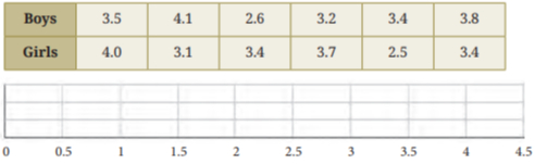

Solution:

To fill the dot plot for the baby weights:
Boys: 3.5, 4.1, 2.6, 3.2, 3.4, 3.8
Girls: 4.0, 3.1, 3.4, 3.7, 2.5, 3.4
Distribution:

{tex}2.5 \mathrm{~kg}: 1 \mathrm{dot}{/tex} (girl)
{tex}2.6 \mathrm{~kg}: 1 \mathrm{dot}{/tex} (boy)
3.1 kg: 1 dot (girl)
3.2 kg: 1 dot (boy)
{tex}3.4 \mathrm{~kg}: 1{/tex} dot (boy), 2 dots (girls)
3.5 kg : 1 dot (boy)
{tex}3.7 \mathrm{~kg}: 1 \mathrm{dot}{/tex} (girl)
3.8 kg: 1 dot (boy)
{tex}4.0 \mathrm{~kg}: 1{/tex} dot (girl)
4.1 kg: 1 dot (boy)

Analysis and Comparison

Both boys and girls have most weights between 3 and 4 kg , showing a healthy clustering for newborns.
The lowest weights are 2.5 kg (girl) and 2.6 kg (boy).
Girls have a repeated value at 3.4 kg , while boys have a slightly wider spread including a maximum at 4.1 kg.
Both groups are similar in average weight, with no significant difference in typical newborn weights shown in this data.

Q.10: The dot plots of heights of another section of Grade 5 students of the same school are shown below. Can you share your observations? What can we infer from the dot plots and the central tendency measures?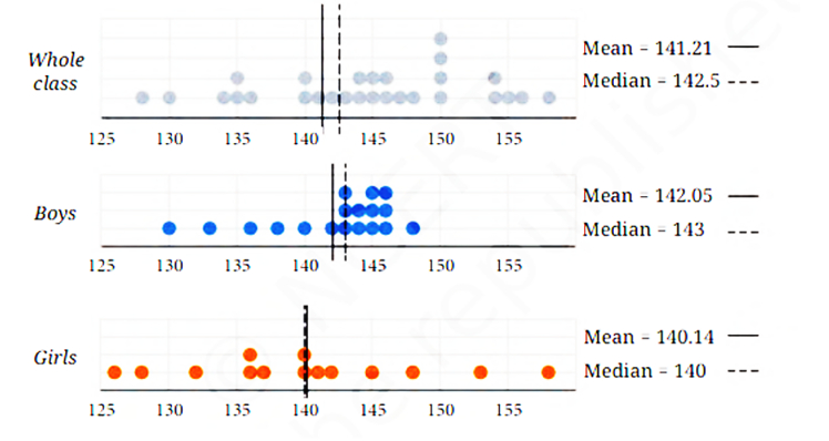

Solution:

Observations from the Dot Plots

Whole class: The dot plot is spread between about 127 cm and 157 cm, with the most common values (clusters) around 140-145 cm.
Boys: Heights slightly cluster more toward the higher end ({tex}140-150 \mathrm{~cm}{/tex}) with a median at 143 cm.
Girls: Most heights cluster around 140 cm , and the plot is more symmetric around this value.

Inferences from Means and Medians

Whole class: The mean (141.21) and median (142.5) are very close, showing the entire class’s heights are balanced without extreme outliers.
Boys vs. Girls: The boys have a slightly higher median (143) and mean (142.05) than the girls (mean {tex}=140.14{/tex}, median {tex}=140{/tex}), indicating boys are on average a little taller than girls in this group.
Central tendency: For both boys and girls, the mean and median are nearly equal, so the data distributions are approximately symmetric for each group.

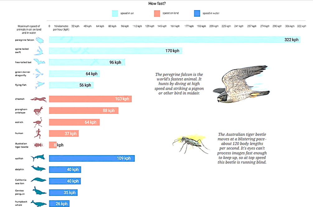
Q.11: The following infographic shows the speeds of a few animals in air, on land, and in water. Can we call this graph a bar graph?

What is the scale used in this graph?
What did you find interesting in this infographic? What do you want to explore further?
Identify a pair of creatures where one’s speed is about twice that of the other.
Can we say that a sailfish is about 4 times faster than a humpback whale? Can we say that a sailfish is the fastest aquatic animal in the world?

Solution:

Yes, the infographic is a bar graph. It uses horizontal bars to visually compare the speeds of animals in air, on land, and in water. Each bar represents the speed of an animal, making comparison easy.

The scale is in kilometres per hour (kph) and each major grid line represents 20 kph increments.
The peregrine falcon is much faster than all other animals listed (322 kph in the air).
The Australian tiger beetle is the fastest among land creatures (around 103 kph). Sailfish (water) can reach 109 kph, which is much quicker than most aquatic animals.
Interesting to further explore: How do these animals achieve such speeds? What adaptations enable the extreme speeds, especially the falcon and beetle?
The pronghorn (88 kph) is about twice as fast as the human (37 kph).
The cheetah (103 kph) is about twice as fast as the kangaroo (55 kph).
Sailfish speed: 109 kph; Humpback whale: {tex}27 \mathrm{kph} .27 \times 4=108{/tex}, so the sailfish is about 4 times faster than the humpback whale.
Based on the chart, the sailfish is the fastest aquatic animal shown. As per current records and this data, it can be considered the fastest known aquatic animal.

Q.12: Preyashi asked her students ‘If you were to get a super power to become aquatic (water-borne), aerial (air-borne), or spaceborne which one would you choose?’. The responses are shown below. Some chose none. Draw a double-bar graph comparing how both grades chose each option. Choose an appropriate scale.

Solution:

Here is a double-bar graph comparing Grade 5 and Grade 9 student preferences for the superpower question (“Aquatic”, “Aerial”, “Spaceborne”, “None”), with each option and grade shown side-by-side. The scale is 1 unit = 2 students.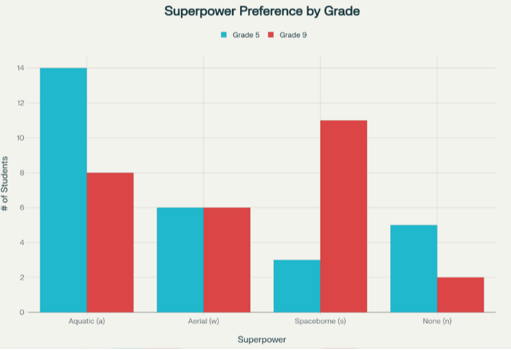

Double-bar graph of superpower choices by Grade 5 and Grade 9

Q.13: The temperature variation over two days in different months in Jodhpur, Rajasthan, is given below. Draw a double-bar graph. Use the scale 1 unit = 4^oC. Can you guess which two months these days might belong to?

Solution:

X-axis: Time (12 am, 3 am, 6 am, 9 am, 12 pm, 3 pm, 6 pm, 9 pm)
Y-axis: Temperature ( {tex}{ }^{\circ} \mathrm{C}{/tex} ), with scale 1 unit {tex}=4^{\circ} \mathrm{C}{/tex}
Draw paired bars for each time slot: one for Day 1 (lower temperatures), one for Day 2 (higher temperatures).

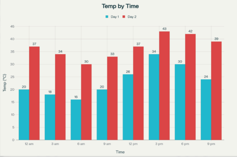
Double-bar graph of temperature variation for two days in Jodhpur
Interpretation

Day 1: Cooler temperatures, typical of a winter or early spring/autumn month.
Day 2: Much hotter, peaking at {tex}43^{\circ} \mathrm{C}{/tex}, typical of a peak summer month (May or June in Rajasthan).

Q.14: The following clustered-bar graph shows the number of electric vehicles registered in some states every year from 2022 to 2024.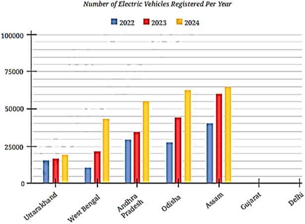

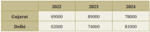
The data (rounded-off to thousands) for the states of Gujarat and Delhi are given in the table below. Mark the corresponding bars on the bar graph. (It is enough if you place the top of the bars between the two appropriate vertical guidelines.)
Notice how the graph is organised, what scale is used, and what patterns the data shows.
Approximately how many more registrations did Assam get in 2023 compared to 2022?
How many times more did the registrations in West Bengal increase from 2022 to 2024?
Is this statement correct — ‘There were very few new registrations in Uttarakhand in 2023 and 2024, as the increase in the bar lengths is minimal’?

Solution:

On the graph, find the relevant columns for Gujarat and Delhi.
For Gujarat, mark the tops at 69,000 (2022), 89,000 (2023), and 78,000 (2024).
For Delhi, mark the tops at 62,000 (2022), 74,000 (2023), and 81,000 (2024).
Because the y-axis uses a scale of 25,000 per main grid line, place each bar between the nearest guidelines above the corresponding state name.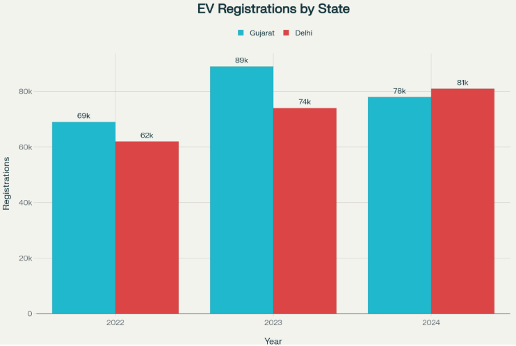

Clustered-bar graph of electric vehicles registered in Gujarat and Delhi (2022-2024)
The graph is clustered: Each state has three adjacent bars (2022, 2023, 2024).
The scale is 25,000 registrations per main vertical grid line.
Bars make it easy to compare states over three years.
Registrations rose sharply in West Bengal, Andhra Pradesh, Odisha, Assam, and Delhi.
Gujarat peaked in 2023, then reduced slightly in 2024.
Uttarakhand saw marginal growth, with little change in bar length.
In 2022, Assam was around 40,000. In 2023, it was about 60,000.
Increase: 60,000-40,000 = 20,00060,000 – 40,000 = 20,000 more registrations in 2023.
2022: {tex}\sim{/tex}13,000; 2024: {tex}\sim{/tex}43,000.
Increase factor: {tex}43,000 \div 13,000 \approx 3.3{/tex}.
Registrations increased a little over three times.
Correct. Uttarakhand shows minimal increase between 2022, 2023, and 2024; the bar heights change only slightly.

Q.15: The dot plots below show the distribution of the number of pockets on clothing for a group of boys and for a group of girls.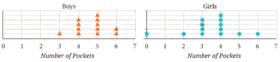

Based on the dot plots, which of the following statements are true?

The data varies more for the boys than for the girls.
The median number of pockets for the boys is more than that for the girls.
The mean number of pockets for the girls is more than that for the boys.
The maximum number of pockets for boys is greater than that for the girls.

Solution:

True. Boys’ pockets range from 3 to 7, with more spread and some isolated higher values. Girls’ pockets cluster mostly between 2 and 5, so variation is less.
True. The boys’ dots cluster around 4-5, while girls’ are around 3-4. The median for boys appears higher.
False. Boys have higher individual maximums, so their mean is at least equal, if not higher, than the girls.
True. Boys reach up to 7 pockets; girls only up to 5.
So, statements (a), (b), and (d) are true according to the dot plots and central tendency measures displayed.

Q.16: The following table shows the points scored by each player in four games: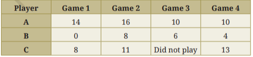

Now answer the following questions:

Find the average number of points scored per game by A.
To find the mean number of points scored per game by C, would you divide the total points by 3 or by 4? Why? What about B?
Who is the best performer?

Solution:

The average number of points scored per game by A :
{tex} \text { Average for } {A}=\frac{14+16+10+10}{4}=12.5 {/tex}
For player C , divide total points {tex}(8+11+13=32){/tex} by 3, not {tex}4-{/tex} since C played only 3 games. For B, divide by 4 (all games played).
A is the best performer, having the highest average score per game (12.5), compared to C ({tex}10.67){/tex} and {tex}\mathrm{B}(4.5){/tex}.

Q.17: The marks (out of 100) obtained by a group of students in a General Knowledge quiz are 85, 76, 90, 85, 39, 48, 56, 95, 81 and 75. Another group’s scores in the same quiz are 68, 59, 73, 86, 47, 79, 90, 93 and 86. Compare and describe both the groups performance using, mean and median.

Solution:

Here is the comparison of the two groups’ performance:
Group 1:
{tex} \text { Mean = 73.0, Median = } 78.5 {/tex}
Group 2:
{tex} \text { Mean }=75.67, \text { Median }=79.0 {/tex}
Description
Group 2 performed slightly better than Group 1, as both the mean and median are higher. This means, on average and for the middle values, Group 2’s scores are greater, indicating overall better performance.

Q.18: Consider this data collected from a survey of a colony.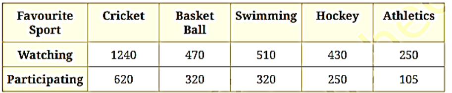

Choose an appropriate scale and draw a double-bar graph. Write down your observations.

Solution:

Here is a double-bar graph comparing the number of people watching and participating in each favorite sport (Cricket, Basket Ball, Swimming, Hockey, Athletics) based on the colony survey data: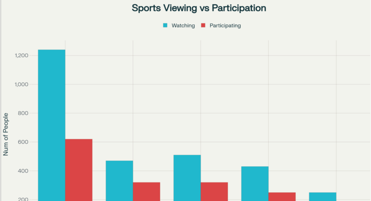

Double-bar graph of Watching vs Participating in Sports (Colony Survey)

Q.19: Consider a group of 17 students with the following heights (in cm): 106, 110, 123, 125, 117, 120, 112, 115, 110, 120, 115, 102, 115, 115, 109, 115, 101. The sports teacher wants to divide the class into two groups so that each group has an equal number of students: one group has students with height less than a particular height and the other group has students with heights greater than the particular height. Suggest a way to do this. Can you guess the age of these students based on the tabular data in the ‘Telling Tall Tales’ section?

Solution:

To divide the class into two groups of equal size, split by the median height:

List all heights in order: 101,102,106,109,110,110,112,115,115,115,115,115,117,120,120,123,125.
The 9th value (median) is 115 cm.
One group: heights < 115 cm (8 students).
Other group: heights {tex}\geq 115 \mathrm{~cm}{/tex} ( 9 students, as there are multiple students at the median value, so the groups are nearly equal).

Likely Age of Students
Based on the heights and the “Telling Tall Tales” context, these students are likely in early/middle primary (around grade {tex}2-4{/tex}), with ages around {tex}7-9{/tex} years old.

Q.20: Describe the mean and median of heights of your class. You can visualise the heights on a dot plot.

Solution: Do it yourself.

Q.21: There are two 7th grade sections at a school. Each section has 15 boys and 15 girls. In one section, the mean height of students is 154.2 cm. From this information, what must be true about the mean height of students in the other section?

The mean height of students in the other section is 154.2 cm.
The mean height of students in the other section is less than 154.2 cm.
The mean height of students in the other section is more than 154.2 cm.
The mean height of students in the other section cannot be determined.

Solution:

The mean height of students in the other section cannot be determined.

There is no data about the other section’s heights, so the mean could be the same, less, or more than 154.2 cm – there is simply not enough information to know.

Q.22: Standing tall in the storm.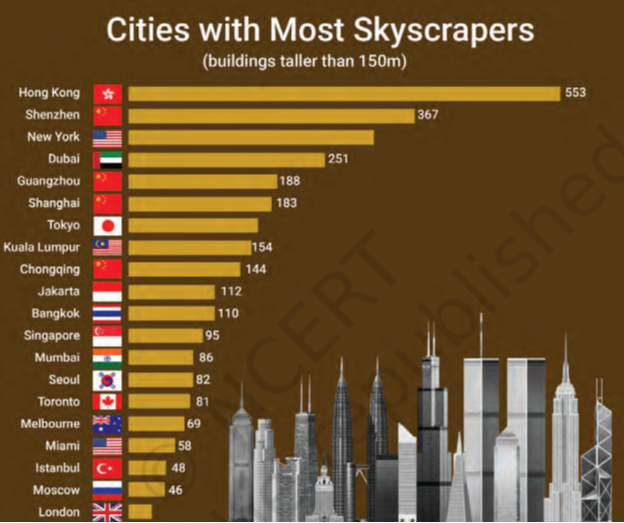

Write estimated values for the number of skyscrapers in New York, Tokyo, and London.
Are the following statements valid?
1. Only 12 cities have more skyscrapers than Mumbai.
2. Only 7 cities have fewer skyscrapers than Mumbai.
3. The tallest building in the world is in Hong Kong.

Solution:

Estimated skyscraper counts
New York: About 295 skyscrapers.
Tokyo: About 163 skyscrapers.
London: About 47 skyscrapers.
Validity of statements
1. Mumbai is ranked 13th on the list with 86 skyscrapers, so 12 cities have more. This statement is valid.
2. There are 20 cities in the chart. Mumbai is at position 13, so 7 cities (from 14th to 20th) have fewer. This statement is valid.
3. The chart shows which city has the most skyscrapers, not the tallest. In fact, the tallest is in Dubai (Burj Khalifa), not Hong Kong. This statement is not valid.

Q.23: Estimate and then measure the objects listed in the following table. Draw a double bar graph based on the data. How accurate were your estimates? Find the average difference between the estimated and measured values.

Object	Estimate (in cm)	Measure (in cm)	Positive Difference
Length of a pen
Length of an eraser
Length of your plam
Length of your geometry box
Length of your math notebook

Solution:

Object	Estimate (cm)	Measure (cm)	Positive Difference
Length of a pen	15	14	1
Length of an eraser	5	4	1
Length of your palm	12	13	1
Length of your geometry box	18	17	1
Length of your math notebook	25	24	1

Calculate Average Difference

Sum all positive differences: {tex}1+1+1+1+1=5{/tex}
Number of objects: 5
Average difference {tex}=5 \div 5=1 \mathrm{~cm}{/tex}

Observation: On average, the estimation was 1 cm off the measured value for each object.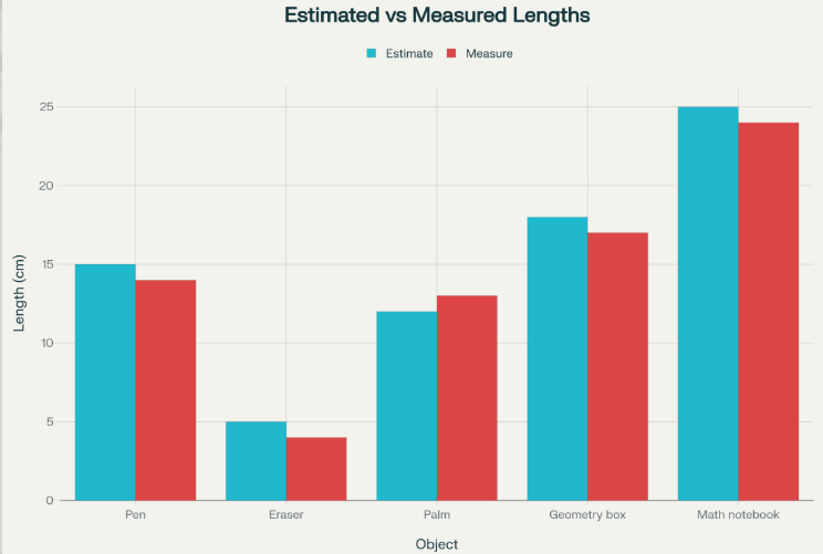

Double-bar graph of estimated versus measured object lengths
This chart allows a clear comparison between your estimation skills and the actual measured values for each item.

Q.24: Aditi likes solving puzzles. She recently started attempting the ‘Easy’ level Sudoku puzzles. The time she took (in seconds) to solve these puzzles are - 410, 400, 370, 340, 360, 400, 320, 330, 310, 320, 290, 380, 280, 270, 230, 220, 240. The first nine values correspond to Week 1 and the rest to Week 2.

Construct a dot plot below showing the data for both weeks.
Describe the mean, median, and any observations you may have about the data.

Solution:

Here is a dot plot showing Aditi’s Sudoku solving times for both weeks. Each dot represents one puzzle-solving time, with blue for Week 1 and red for Week 2. This visualizes her improvement and the distribution of her scores.
[Dot plot of Sudoku solving times for Weeks 1 and 2]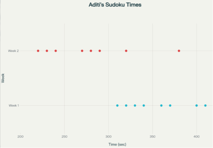

Dot plot of Sudoku solving times for Weeks 1 and 2
The mean time to solve the puzzles is about 322 seconds, while the median time is 320 seconds.
Both values are very close, showing that most of Aditi’s solving times cluster around this range.
Observations
- In Week 1, Aditi took longer to solve the puzzles, with most times between 310 and 410 seconds.
- In Week 2, Aditi consistently solved puzzles faster, with times between 220 and 380 seconds.
- The dot plot displays a clear improvement in speed and more consistency in Week 2.
- The data suggests Aditi became quicker with practice, and her puzzle-solving times became less spread out.

Q.25: Individual Project: Pick at least one of the following:

How Long is a Sentence? Pick any two textbooks from different subjects. Choose any page with a lot of text from each book.
1. Use a dot plot to describe how many words the sentences have on each page.
2. Compare the data of both the pages using mean and median.
What is in a Name? Write down the names of all of your classmates. The following are some interesting things you can do with this data!
1. Find the mean and median name length (number of letters in a name).
2. Visualise the data and describe its variability and central tendency.
Which starting letters are more popular? Which are less popular?
What is the median starting letter? What does this say about the number of names starting with the letters A - M and N - Z?
Plot a double-bar graph showing the number of boys’ names and girls’ names that:
- start and end with vowels,
- start with vowels and end with consonants,
- start and end with consonants.

Solution: Do it yourself.

Q.26: Individual project (long term): This requires collecting data over 2 weeks or more.
In and Out: Track how many times you step out of your house in a day. Do this for a month.

Describe the variability and central tendency of this data. Make a dot plot.
Do you find anything interesting about this data? Share your observations.
You can ask any of your family members or friends to do this as well.

Solution: Do it Yourself.

Q.27: Small-group project: Pick at least one of the following. Make groups of 8 to 10. Collect data individually as needed. Put together everyone’s data and do the appropriate analysis and visualisation.

Our heights vs. our family’s heights: Collect the heights of your family members.
1. Make a dot plot showing heights of just your family members. Describe its variability and central tendency.
2. Make a double-bar graph showing each student’s height next to their family’s mean height.
3. Look at everyone’s data and share your observations.
Estimating time: Check the time and close your eyes. Open them when you think 1 minute has passed (no counting). Note down after how m-any seconds you opened your eyes. Collect this data for yourself and for your family members. Repeat this activity to estimate 3 minutes.
1. Make two dot plots (for 1 minute and 3 minutes) showing estimates of just your family members.
2. Mark these on the respective dot plots. Describe its variability and central tendency.
3. Make a double bar graph showing each family’s mean 1 minute estimate and mean 3 minute estimate.
4. Look at everyone’s data and share your observations.