Tales by dots and lines – NCERT Solutions Class 8 Maths (Ganita Prakash) includes all the questions with solutions given in the NCERT Class 8 Maths (Ganita Prakash).
NCERT Solutions Class 8
English Poorvi Hindi Malhar Maths Ganita Prakash Science Curiosity Social Exploring SocietyTales by dots and lines – NCERT Solutions
Q.1: Consider any 2 numbers. Find their average/arithmetic mean. Repeat this by taking other pairs. What do you observe?
For example, let the two numbers be 3 and 7. Their average is {tex}\frac{3+7}{2}=5{/tex}. Taking another pair of numbers, say 8 and 9, their average is {tex}\frac{8+9}{2}=8.5{/tex}. Visualising these as dot plots we get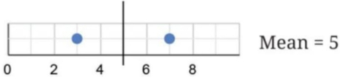
Solution:
Let’s take different pairs of numbers and find their averages:
Pair 1: 3 and 7 Average {tex}=(3+7) \div 2=10 \div 2=5{/tex}
Pair 2: 8 and 9 Average {tex}=(8+9) \div 2=17 \div 2=8.5{/tex}
Pair 3: 10 and 20 Average {tex}=(10+20) \div 2=30 \div 2=15{/tex}
Pair 4:5 and 15 Average {tex}=(5+15) \div 2=20 \div 2=10{/tex}
Observation: The mean (average) is always exactly halfway between the two numbers. The distance from the smaller number to the mean equals the distance from the mean to the larger number.
Q.2: Calculate and mark the mean of each collection of data below.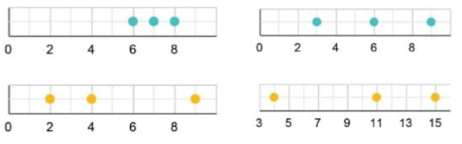
Solution:
- Collection: 5, 7,9
{tex} \text { Mean }=(5+7+9) \div 3=21 \div 3=7 {/tex}
The mean is 7. - Collection: 2, 4, 6, 8
{tex} \text { Mean }=(2+4+6+8) \div 4=20 \div 4=5 {/tex}
The mean is 5. - Collection: 10, 10, 11, 17
{tex} \text { Mean }=(10+10+11+17) {/tex}{tex}\div 4=48 \div 4=12 {/tex}
The mean is 12.
Q.3: Can you explain how the mean is the centre of each collection?
Solution:
The mean is the centre because the sum of distances of all points to the left of the mean equals the sum of distances of all points to the right of the mean.
For example, in collection {tex}(c): 10,10,11,17{/tex} with mean {tex}=12{/tex}:
- Distance on left: {tex}(12-10)+(12-10)+{/tex}{tex}(12-11)=2+2+1=5{/tex}
- Distance on right: {tex}(17-12)=5{/tex}
Both distances are equal (5 units each), showing the mean balances the data.
Q.4: Mark the mean for the collections below.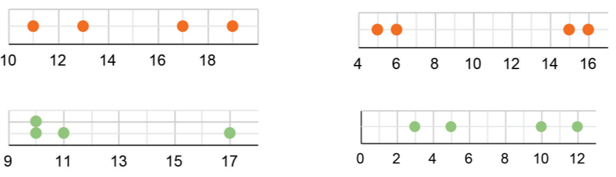
Solution:
- Collection: 3, 5, 7, 9, 11
{tex} \text { Mean }=(3+5+7+9+11) {/tex}{tex}\div 5=35 \div 5=7 {/tex} - Collection: 1, 3, 5, 7
{tex} \text { Mean }=(1+3+5+7){/tex}{tex} \div 4=16 \div 4=4 {/tex}
Q.5: Can you explain how the mean is the centre of each collection?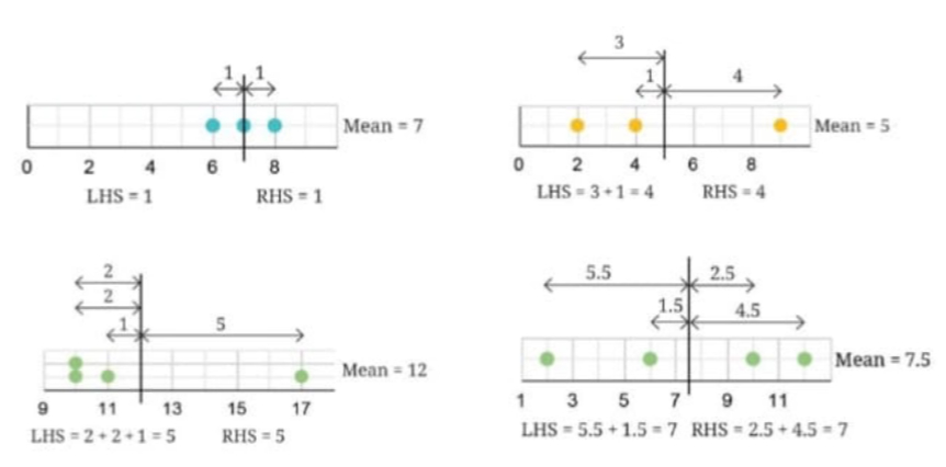
Solution:
For collection (a): 3, 5, 7, 9, 11 with mean {tex}=7{/tex}:
- Distances on left: {tex}(7-3)+(7-5)=4+2=6{/tex}
- Distances on right: {tex}(9-7)+(11-7)=2+4=6{/tex}
For collection (b): 1,3,5,7 with mean {tex}=4{/tex} :
- Distances on left: {tex}(4-1)+(4-3)=3+1=4{/tex}
- Distances on right: {tex}(5-4)+(7-4)=1+3=4{/tex}
In both cases, the total distances on both sides are equal, confirming the mean is the centre.
Q.6: Can you explain how the mean is the centre of each collection?
Is the mean the midpoint of the two endpoints/extremes of the data?
Solution:
No, the mean is not always the midpoint of the two extremes.
For example, in the collection 10, 10, 11, 17:
- Midpoint of extremes {tex}=(10+17) \div 2=27 \div 2=13.5{/tex}
- Mean = 12
The mean (12) is different from the midpoint of extremes (13.5).
Instead, the mean is the point where the sum of distances on the left equals the sum of distances on the right.
Q.7: Can there be more than one such ‘centre’? In other words, is there any other value such that the sum of the distances to the values lower than it and the values higher than it will still be equal?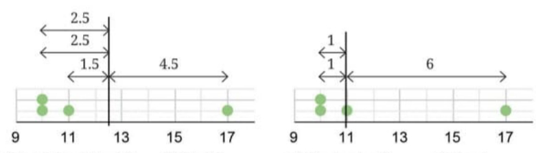
Solution:
No, there cannot be more than one such centre.
Proof: Consider the collection {tex}10,10,11,17{/tex} with mean {tex}=12{/tex}.
If we take any value greater than 12:
- All distances on the left side will increase
- All distances on the right side will decrease
- The balance is broken
If we take any value less than 12:
- All distances on the left side will decrease
- All distances on the right side will increase
- Again, the balance is broken
Therefore, there is only one unique centre (the mean) where the sum of distances on both sides is equal.
Q.8: Will including a new value in the data increase or decrease the mean?
When a new value greater than the mean is included, the mean increases to maintain the balance between the sum of distances on the LHS and RHS, as illustrated below.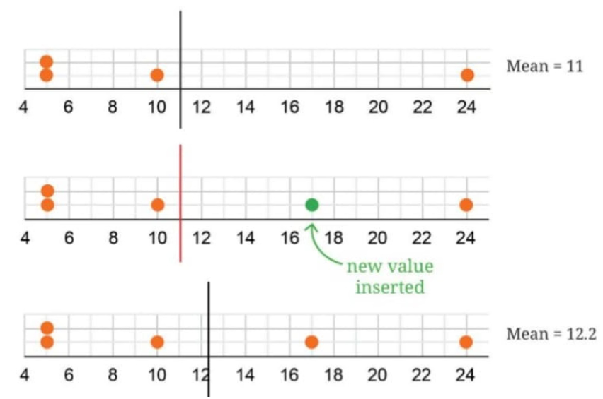
Solution:
It depends on the value being included:
- If the new value is greater than the current mean: The mean will increase.
- Example: Data: {tex}4,6,8({/tex} mean {tex}=6){/tex}
- Adding 10: New data: 4, 6, 8, 10
- New mean {tex}=(4+6+8+10) \div 4=28 \div 4=7{/tex}
- The mean increased from 6 to 7.
- If the new value is less than the current mean: The mean will decrease.
- Example: Data: {tex}4,6,8({/tex} mean {tex}=6){/tex}
- Adding 2: New data: 2,4,6,8
- New mean {tex}=(2+4+6+8) \div 4=20 \div 4=5{/tex}
- The mean decreased from 6 to 5.
- If the new value equals the mean: The mean will remain the same.
Q.9: What happens to the mean if a value equal to the mean is included or removed?
Solution:
Including a value equal to the mean: The mean remains unchanged.
- Example: Data: {tex}3,5,7{/tex} (mean {tex}=5{/tex} )
- Adding 5: New data: 3,5,5,7
- New mean {tex}=(3+5+5+7) \div 4=20 \div 4=5{/tex}
- Mean stays 5.
Removing a value equal to the mean: The mean remains unchanged.
- Example: Data: {tex}3,5,5,7{/tex} (mean {tex}=5{/tex})
- Removing 5: New data: 3, 5, 7
- New mean {tex}=(3+5+7) \div 3=15 \div 3=5{/tex}
- Mean stays 5.
Fair-share interpretation: When we include or remove a value equal to the mean, we’re not changing the “fair share” amount. Each person already has their fair share, so adding or removing someone with exactly the fair share doesn’t change what everyone else has.
Q.10: Explore if it is possible to include or remove 2 values such that the mean is unchanged.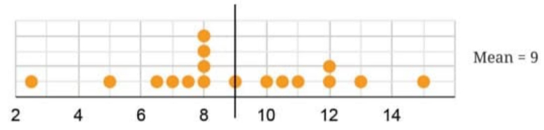
Solution:
Yes, this is possible if the total of the three values equals 3 times the mean.
Example: Data: 5, 7, 9 (mean {tex}=7{/tex})
To keep mean at 7:
- We need 3 values that total to {tex}3 \times 7=21{/tex}
- Include 4,6 (both less than 7) and 11 (greater than 7)
- Check: {tex}4+6+{1 1}=2 {1}{/tex}
- New data: 4, 5, 6, 7, 9, 11
- New mean {tex}=(4+5+6+7+9+11) \div 6{/tex} {tex}=42 \div 6=7{/tex}
Q.11: Try to include 2 values greater than the mean and 1 value less than the mean, so that the mean stays the same.
Solution:
Example: Data: {tex}5,7,9({/tex}mean {tex}=7){/tex}
To keep mean at 7:
- We need 3 values that total to {tex}3 \times 7=21{/tex}
- Include 8, 10 (both greater than 7) and 3 (less than 7)
- Check: {tex}8+10+3=21{/tex}
- New data: 3, 5, 7, 8, 9, 10
- New mean {tex}=(3+5+7+8+9+10){/tex}{tex} \div 6=42 \div 6=7{/tex}
Relatively Unchanged!
Q.12: Consider the data: 8, 3, 10, 13, 4, 6, 7, 7, 8, 8, 5. Calculate its mean.
Solution:
{tex}{ Sum }=8+3+10+{/tex}{tex}13+4+6+7+7+8+8+5=79 {/tex}
Number of values {tex}=11{/tex}
Mean {tex}=79 \div 11=7.18{/tex} (approximately)
Q.13: Now, consider this data with every value increased by {tex}10: 18,13,20,23,14{/tex}, {tex}16,17,17,18,18,15{/tex}. What is its mean? Is there a quicker way to find out?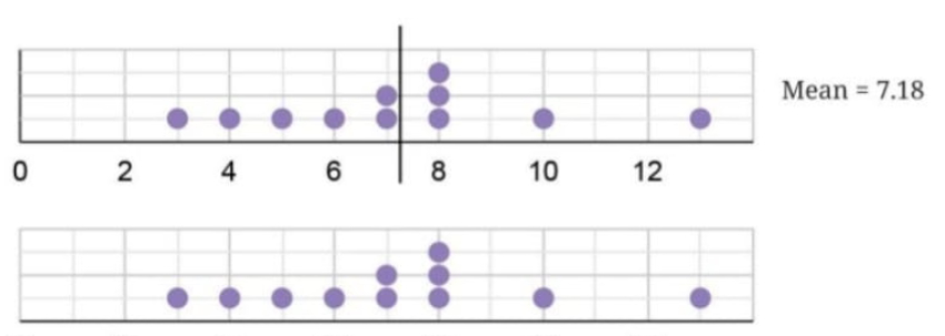
Solution:
Method 1: (Direct calculation): Sum {tex}=18+13+20+23+14+{/tex}{tex}16+17+17+ 18+18+15=189{/tex}
Mean {tex}=189 \div 11=17.18{/tex} (approximately)
Method 2: (Quicker way): Since every value increased by 10, the mean also increases by 10.
New mean= Original mean {tex}+10=7.18+10=17.18{/tex}
This is much quicker!
Observation: The relative position of the mean stays the same. The entire data set shifts up by 10, so the mean also shifts up by 10.
Q.14: Try to explain, using algebra, what the average is when a fixed number, e.g., 2 is subtracted from every value in the collection.
Solution:
Let there be {tex}n{/tex} values: {tex}x_1, x_2, x_3, \ldots x_n{/tex}
Original average {tex}=\left(x_1+x_2+x_3+\ldots+x_n\right) \div n=a{/tex}
When 2 is subtracted from every value:
New average {tex}=\left[\left({x}_1-2\right)+\left({x}_2-2\right)+\left({x}_3-2\right)+\ldots+\left({x}_{{n}}-2\right)\right] \div {n}{/tex}
{tex} =\left[x_1+x_2+x_3+\ldots+x_n-2 n\right] \div n {/tex}
{tex} =\left[\left(x_1+x_2+x_3+\ldots+x_n\right) \div n\right]-(2 n \div n) {/tex}
{tex} =a-2 {/tex}
Therefore, the new average is 2 less than the original average.
Q.15: Try to explain this using the fair-share interpretation of average that you learnt last year.
Solution:
Using the fair-share interpretation:
If everyone has their fair share (the average), and then everyone gives away 2 units, the new fair share will be the old fair share minus 2.
For example: If 4 friends share 20 chocolates equally, each gets 5 chocolates (fair share {tex}=5{/tex}).
If each friend gives away 2 chocolates, they now have {tex}20-(4 \times 2)=12{/tex} chocolates total.
New fair share {tex}=12 \div 4=3=5-2{/tex}
The fair share decreased by exactly 2.
Q.16: What happens to the average if every value in the collection is doubled?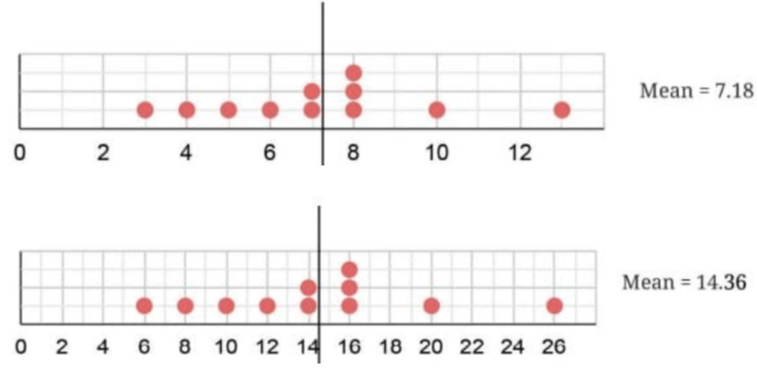
Solution:
The average also doubles.
Example: Consider data: 3, 5, 7
Original mean {tex}=(3+5+7) \div 3=15 \div 3=5{/tex}
Doubled data: 6, 10, 14
New mean {tex}=(6+10+14) \div 3=30 \div 3=10{/tex}
New mean {tex}=2 \times{/tex} Original mean
Algebraic Proof:
Let the {tex}n{/tex} values be {tex}x_1, x_2, x_3, \ldots x_n{/tex} with average {tex}a{/tex}.
Original average: {tex}\left(x_1+x_2+x_3+\ldots+x_n\right) \div n=a{/tex}
When every value is multiplied by 5:
New average {tex}=\left[\left(5 x_1\right)+\left(5 x_2\right)+\left(5 x_3\right)+\ldots+\left(5 x_n\right)\right] \div n{/tex}
{tex} =\left[5\left(x_1+x_2+x_3+\ldots+x_n\right)\right] \div n{/tex}{tex} \text { (using distributive property) } {/tex}
{tex} =5 \times\left[\left(x_1+x_2+x_3+\ldots+x_n\right) \div n\right] {/tex}
{tex} =5 \times a {/tex}
{tex} =5 a {/tex}
Therefore, when every value is multiplied by 5, the new average is 5 times the original average.
Similarly, when every value is doubled, the average also doubles.
Q.17: Will including a new value to the data increase or decrease the median?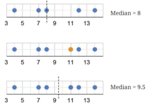
Solution:
Let’s consider the data: {tex}3,5,7,8,10,11,13{/tex}
The median is 8 (middle value).
Case 1: Including a value greater than the median (e.g., 11)
New data: 3, 5, 7, 8, 10, 11, 11, 13
Since we now have 8 values (even), the median {tex}={/tex} average of 4th and 5th values Median {tex}= (8+10) \div 2=9{/tex}
The median increased from 8 to 9.
Case 2: Including a value less than the median(e.g.,4)
New data: 3, 4, 5, 7, 8, 10, 11, 13
Median {tex}=(7+8) \div 2=7.5{/tex}
The median decreased from 8 to 7.5.
Conclusion:
- Including a value greater than the median {tex}\rightarrow{/tex} median increases
- Including a value less than the median {tex}\rightarrow{/tex} median decreases
- Including a value equal to the median {tex}\rightarrow{/tex} median stays the same (usually)
Q.18: Coach Balwan noted down the weights of the kushti players (wrestlers) and the mean as shown. But one value that was written down got smudged. Can you find out the missing value?
Given: Weights: 42, 40, 39, 33, 48, 38, 42, 35, 32, w
Mean = 39.2 kg
Solution:
We know: Mean = Sum of all values {tex}\div{/tex} Number of values
{tex} 39.2=(42+40+39+33+48{/tex}{tex}+38+42+35+32+w) \div 10 {/tex}
{tex} 39.2=(349+w) \div 10 {/tex}
Multiplying both sides by 10:
{tex} 392=349+w {/tex}
{tex} w=392-349=43 {/tex}
The missing value is {tex}{4 3 ~ k g}{/tex}.
Q.19: Venkayya keeps track of the coconut harvest in his farm. He calculates the average harvest per tree as 25.6 . His son verifies the counts and finds that one tree’s harvest count is incorrectly noted as 3 more than the actual number. Can you find the correct average if the number of trees is 15?
Solution:
Given:
- Number of trees {tex}=15{/tex}
- Incorrect average {tex}=25.6{/tex}
- One tree’s count is 3 more than actual
Step 1: Find the incorrect total harvest
Average {tex}={/tex} Total harvest {tex}\div{/tex} Number of trees
{tex}25.6={/tex} Total harvest {tex}\div 15{/tex}
Total harvest (incorrect) {tex}=25.6 \times 15=384{/tex} coconuts
Step 2: Find the correct total harvest
Since one tree’s count is 3 more than actual:
Correct total {tex}=384-3=381{/tex} coconuts
Step 3: Find the correct average
Correct average {tex}=381 \div 15=25.4{/tex}
The correct average harvest is 25.4 coconuts per tree.
Q.20: What is the average family size of students in your class? How would you find this out?
| Number | Frequency |
| 3 | 3 |
| 4 | 11 |
| 5 | 9 |
| 6 | 7 |
| 7 | 3 |
| 8 | 1 |
| 9 | 1 |
| 10 | 1 |
Solution:
Incorrect approach: {tex}(3+4+5+6+7{/tex}{tex}+8+9+10) \div 8=6.5{/tex}
This is wrong because it doesn’t account for how many times each value occurs.
Correct approach:
Mean {tex}={/tex} Sum of all values ÷ Total number of values
Sum of all values {tex}=(3 \times 3)+(4 \times 11)+(5 \times 9)+{/tex}{tex}(6 \times 7)+(7 \times 3)+(8 \times 1){/tex}{tex}+(9 \times 1)+(10 \times 1){/tex}
{tex} =9+44+45+42+21+8+9+10 {/tex}
{tex} \text { = } 188 {/tex}
Total number of values {tex}=3+11+9+7+3+1+1+1=36{/tex}
{tex} \text { Mean }=188 \div 36=5.22 \text { (approximately) } {/tex}
The average family size is 5.22.
Q.21: What is the median family size of this class?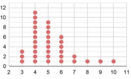
Solution:
Total number of students {tex}=36{/tex}
Since 36 is even,the median will bethe average ofthe 18th and 19th values when data is arranged in order.
Let’s add frequencies progressively:
- Values 1 to 3: family size 3 (frequency 3)
- Values 4 to 14: family size 4 (frequency 11, cumulative {tex}=14{/tex})
- Values 15 to 23: family size 5 (frequency 9, cumulative {tex}=23{/tex})
The 18th and 19th values both fall inthe range where family size {tex}=5{/tex}.
Therefore, median {tex}={5}{/tex}.
Q.22: Can you tell which cell has the marks obtained by Farooq in Mathematics?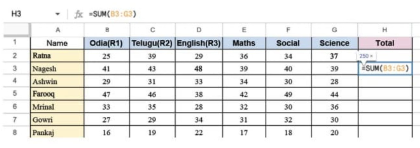
Solution:
Farooq’s marks in Mathematics are in cell E5.
(Column E = Mathematics, Row 5 = Farooq)
Q.23: Can you tell what data is in column B7?
Solution:
Column B is for Odia marks, and Row 7 is for Gowri.
Therefore, cell B7 contains Gowri’s marks in Odia = 27.
Q.24: In which subjects has Ashwin scored more than 30 marks?
Solution:
Ashwin is in Row 4. Let’s check his marks:
- Odia: 29 (not > 30)
- Telugu: 31 (> 30)
- English: 33 (> 30)
- Maths: 34 (> 30)
- Social Science: 30 (not > 30)
- Science: 28 (not > 30)
Ashwin scored more than 30 marks in Telugu, English, and Maths.
Q.25: What formula would you type to find out the class average marks in Science?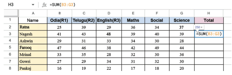
Solution:
Science marks are in column G, from rows 2 to 23.
Formula: = AVERAGE(G2:G23)
This will calculate the average of all Science marks in the class.
Q.26: Find out if the class average marks in Odia is greater than the class average marks in Telugu.
Solution:
Formula for Odia average: = AVERAGE(B2:B23) Formula for Telugu average:
= AVERAGE(C2:C23)
When calculated:
- Odia average {tex}\approx 30.23{/tex}
- Telugu average {tex}\approx 32.68{/tex}
No, the class average marks in Odia (30.23) is less than the class average marks in Telugu (32.68).
Q.27: Find the mean of the following data and share your observations:
- The first 50 natural numbers.
- The first 50 odd numbers.
- The first 50 multiples of 4.
Solution:
- The first 50 natural numbers are: {tex}1,2,3,4, \ldots, 50{/tex}
Sum of first n natural numbers {tex}={n}({n}+1) \div 2{/tex}
{tex} \text { Sum }=50 \times 51 \div 2=2550 \div 2=1275 {/tex}
{tex} \text { Mean }=1275 \div 50=25.5 {/tex}
Observation: The mean of the first {tex}{n}{/tex} natural numbers is always {tex}({n}+{1}) \div 2{/tex}. For 50 numbers, it’s {tex}51 \div 2=25.5{/tex}. - The first 50 odd numbers are: {tex}1,3,5,7, \ldots, 99{/tex}
Sum of first {tex}{n}{/tex} odd numbers {tex}={n}^2{/tex}
Sum {tex}=50^2=2500{/tex}
{tex} \text { Mean }=2500 \div 50=50 {/tex}
Observation: The mean of the first {tex}n{/tex} odd numbers is always {tex}n{/tex}. For 50 odd numbers, the mean is 50. - The first 50 multiples of 4 are: {tex}4,8,12,16, \ldots, 200{/tex}
This is 4 times the first 50 natural numbers.
Sum {tex}=4 \times({/tex}sum of first 50 natural numbers{tex})=4 \times 1275=5100{/tex}
Mean {tex}=5100 \div 50=102{/tex}
Observation: The mean of the first {tex}{n}{/tex} multiples of 4 is 4 times the mean of the first {tex}{n}{/tex} natural numbers. Mean {tex}=4 \times 25.5=102{/tex}.
Q.28: The dot plot below shows a collection of data and its average; but one dot is missing. Mark the missing value so that the mean is 9 (as shown below).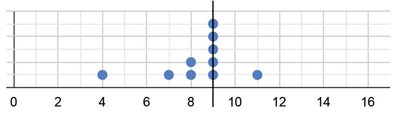
Solution:
From the dot plot, visible values are: {tex}7,8,8,9,10,11,12{/tex}
Let the missing value be x.
Given: Mean {tex}=9{/tex}
{tex} 9=(7+8+8+9+10+11+12+x) \div 8 {/tex}
{tex} 9=(65+x) \div 8 {/tex}
{tex} 72=65+x {/tex}
{tex} x=72-65=7 {/tex}
The missing value is 7
The missing dot should be marked at position 7 on the number line.
Q.29: Sudhakar, the class teacher, asks Shreyas to measure the heights of all 24 students in his class and calculate the average height. Shreyas informs the teacher that the average height is 150.2 cm. Sudhakar discovers that the students were wearing uniform shoes when the measurements were taken and the shoes add 1 cm to the height.
- Should the teacher get all the heights measured again without the shoes to find the correct average height? Or is there a simpler way?
- What is the correct average height of the class?
- 174.2 cm
- 126.2 cm
- 150.2 cm
- 149.2 cm
- 51.2 cm
- None of the above
- Insufficient information
Solution:
- No, the teacher doesn’t need to measure all heights again.
Simpler way: Since every student was wearing shoes that add 1 cm to their height, every measurement is 1 cm more than it should be. Therefore, the average height is also 1 cm more than it should be.
Correct average height = Measured average height – {tex}1 {~cm}=150.2-1=149.2 {~cm}{/tex} - (d) 149.2 cm
Explanation: When a fixed amount (1 cm) is added to every value, the average also increases by that same amount. Conversely, when we subtract 1 cm from every measurement, the average also decreases by 1 cm.
Q.30: The three dot plots below show the lengths, in minutes, of songs of different albums. Which of these has a mean of 5.57 minutes? Explain how you arrived at the answer.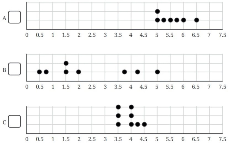
Solution:
To find which album has a mean of 5.57 minutes, we need to calculate the mean for each dot plot
Album A: Let’s count the dots and their positions:
- At 4: 2 dots
- At 5: 5 dots
- At 6: 3 dots
- At 7: 2 dots
{tex} 5 {um}=(4 \times 2)+(5 \times 5)+{/tex}{tex}(6 \times 3)+(7 \times 2)=8+25+18+14=65 {/tex}
Number of songs {tex}=2+5+3+2=12{/tex}
Mean {tex}=65 \div 12=5.42{/tex} minutes (approximately)
Album B:
- At 3 : 1 dot
- At 4 : 2 dots
- At 5 : 3dots
- At 6 : 4 dots
- At 7 : 4 dots
{tex} 5 {um}=(3 \times 1)+(4 \times 2)+{/tex}{tex}(5 \times 3)+(6 \times 4)+{/tex}{tex}(7 \times 4)=3+8+15+24+28=78 {/tex}
Number of songs {tex}=1+2+3+4+4=14{/tex}
Mean {tex}=78 \div 14=5.57{/tex} minutes
Album C:
- At 4: 4 dots
- At 5: 3dots
- At 6:4 dots
- At 7: 1 dot
{tex}{Sum}=(4 \times 4)+(5 \times 3)+{/tex}{tex}(6 \times 4)+(7 \times 1){/tex} {tex}=16+15+24+7=62{/tex}
Number of songs {tex}=4+3+4+1=12{/tex}
Mean {tex}=62 \div 12=5.17{/tex} minutes (approximately)
Answer: Album {tex}B{/tex} has a mean of 5.57 minutes.
Q.31: Find the median of {tex}8,10,19,23,26,34,40,41,41,48,51,55,70{/tex}, 84, 91, 92.
- If we include one value to the data (in the given list) without affecting the median, what could that value be?
- If we include two values to the data without affecting the median what could the two values be?
- If we remove one value from the data without affecting the median what could the value be?
Solution:
The data is already in ascending order.
Number of values {tex}=16{/tex} (even)
Median {tex}={/tex} Average of 8th and 9th values
8 th value {tex}=41{/tex} th value {tex}=41{/tex}
Median {tex}=(41+41) \div 2=82 \div 2=41{/tex}
- To keep the median at 41, the new value should be 41 itself.
When we add 41, the data becomes: {tex}8,10,19,23,26,34,40,41{/tex}{tex},41,41,48,51,55,70{/tex}, 84,91,92 (17 values)
The 9th value (middle value) is still 41.
Median remains 41 - We can include any two values such that one is {tex}\leq 41{/tex} and the other is {tex}\geq 41{/tex}.
Example 1: Include 30 and 50 New data: {tex}8,10,19,23,26,30,34,40{/tex}{tex},41,41,48,50,51{/tex}, {tex}55,70,84,91,92(18{/tex} values{tex}){/tex}
Median {tex}=(41+41) \div 2=41{/tex}
Example 2: Include 41 and 41
New data has 18 values with 9th and 10th both being 41
Median = 41 - We can remove any value except 41.
Example: Remove 8
New data: {tex}10,19,23,26,34,40,41,{/tex}{tex}41,48,51,55,70,84,91,92{/tex} (15 values)
Median {tex}=8{/tex}th
value {tex}=41{/tex}
Or remove 92 : New data: {tex}8,10,19,23,26,34,40,{/tex}{tex}41,41,48,51,55,70,84,91{/tex} (15 values) Median {tex}=8{/tex}th
value {tex}=41{/tex}
Q.32: Examine the statements below and justify if the statement is always true, sometimes true, or never true.
- Removing a value less than the median will decrease the median.
- Including a value less than the mean will decrease the mean.
- Including any 4 values will not affect the median.
- Including 4 values less than the median will increase the median.
Solution:
- Sometimes true.
Example when true: Data: {tex}1,2,3,4,5{/tex} (median = 3)
Remove 1: New data: {tex}2,3,4,5{/tex} (median = 3.5)
The median increased (not decreased), so this shows it’s not always true.
Example when false: Data: {tex}1,3,5,7,9{/tex} (median {tex}=5){/tex}
Remove 1: New data: 3,5,7,9 {tex}({/tex}median {tex}=6){/tex}
The median increased.
Conclusion: The statement is sometimes true depending on the position and distribution of values. - Always true.
When we include a value less than the mean, the total sum increases by less than the mean amount, but the count increases by 1. This causes the average to decrease.
Example: Data: {tex}4,6,8({/tex} mean {tex}=6){/tex} Include {tex}2({/tex} which is {tex}<6){/tex} : New data: {tex}2,4,6,8{/tex}
New mean {tex}= 20 \div 4=5{/tex}
The mean decreased from 6 to 5 - Sometimes true.
Example when true: Data: {tex}10,20,30,40,50({/tex}median {tex}=30){/tex}
Include: {tex}15,25,35,45{/tex}
New data: {tex}10,15,20,25,30,35,40,45,50(9{/tex} value{tex}){/tex}
Median {tex}=30{/tex}
Example when false: Data: {tex}10,20,30{/tex} (median {tex}=20){/tex} Include: {tex}1,2,3,4 {/tex}
New data: {tex}1,2,3,4{/tex}, 10,20,30 (7 values)
Median = 4 (changed!)
Conclusion: Sometimes true, depending on what values are included. - Never true.
Including values less than the median will either keep the median the same or decrease it, but it will never increase it.
Example: Data: 10,20,30,40,50 (median = 30)
Include: 5,8,12,15 (all < 30)
New data: 5, {tex}8,10,12,15,20,30,40,50(9{/tex} values{tex}){/tex}
Median {tex}=15({/tex} decreased! {tex}){/tex}
Q.33: The mean of the numbers 8, 13, 10, 4, 5, 20, y, 10 is 10.375. Find the value of y.
Solution:
Mean {tex}={/tex} Sum of all values {tex}\div{/tex} Number of values
{tex} 10.375=(8+13+10+4{/tex}{tex}+5+20+y+10) \div 8 {/tex}
{tex} 10.375=(70+y) \div 8 {/tex}
Multiplying both sides by 8:
{tex} 83=70+y {/tex}
{tex} y=83-70=13 {/tex}
The value of y is 13.
Verification: {tex}(8+13+10+4+5+20+13+10){/tex}{tex} \div 8=83 \div 8=10.375{/tex}
Q.34: The mean of a set of data with 15 values is 134. Find the sum of the data.
Solution:
Mean = Sum of data {tex}\div{/tex} Number of values
{tex} 134=\text { Sum } \div 15 {/tex}
{tex} \text { Sum }=134 \times 15=2010 {/tex}
The sum of the data is 2010.
Q.35: Consider the data: {tex}12,47,8,73,18,35,39,8,29,25, p{/tex}. Which of the following number(s) could be {tex}p{/tex} if the median of this data is 29?
- 10
- 25
- 40
- 100
- 29
- 47
- 30
Solution:
The data has 11 values, sothe median will bethe 6th value when arranged in order.
First, let’s arrangethe known values: {tex}8,8,12,18,25,29,35,39,47,73{/tex}
We needthe 6th value to be 29.
Currently without p, in order: {tex}8,8,12,18,25,29,35,39,47,73{/tex}
Testing each option:
- {tex}{p}={1 0 : A rr a n g e d}:{/tex}{tex} 8,8,10,12,18,25,29,35,39,47,73{/tex}
6th value {tex}=25{/tex} - {tex}{p}={2 5}{/tex} :Arranged: {tex}8,8,12,18,25,25,29,35,39,47,73{/tex}
6th value {tex}=25{/tex} - {tex}{p}={4 0}{/tex} :Arranged: {tex}8,8,12,18,25,29,35,39,40,47,73{/tex}
6th value {tex}=29{/tex} - {tex}{p}={1 0 0}:{/tex} Arranged: {tex}8,8,12,18,25,29,35,39,47,73,100{/tex}
6th value {tex}=29{/tex} - p = 29:Arranged: {tex}8,8,12,18,25,29,29,35,39,47,73{/tex}
6th value {tex}=29{/tex} - {tex}{p}={4 7}:{/tex} Arranged: {tex}8,8,12,18,25,29,35,39,47,47,73{/tex}
6th value {tex}=29{/tex} - p = 30:Arranged: {tex}8,8,12,18,25,29,30,35,39,47,73{/tex}
6th value {tex}=29{/tex}
Answer: (iii) 40, (iv) 100, (v) 29, (vi) 47, (vii) 30
All these values keepthe median at 29 because they are all {tex}\geq 29{/tex}, sothe 6th position remains 29.
Q.36: The number of times students rode their cycles in a week is shown in the dot plot below. Four students rode their cycles twice in that week.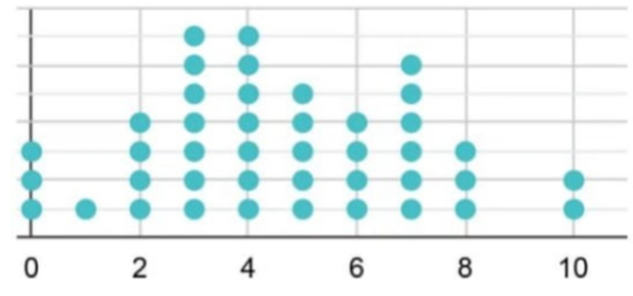
- Find the average number of times students rode their cycles.
- Find the median number of times students rode their cycles.
- Which of the following statements are valid? Why?
- Everyone used their cycle at least once.
- Almost everyone used their cycle a few times.
- There are some students who cycled more than once on some days.
- Exactly 5 students have used their cycles more than once on some days.
- The following week, if all of them cycled 1 more time than they did the previous week, what would be the average and median of the next week’s data?
Solution:
- From the dot plot:
- 0 times: 2 students
- 1 time: 3 students
- 2 times: 4 students
- 3 times: 5 students
- 4 times: 3 students
- 5 times: 2 students
- 6 times: 1 student
Sum {tex}=(0 \times 2)+(1 \times 3)+(2 \times 4)+(3 \times 5)+{/tex}{tex}(4 \times 3)+(5 \times 2)+(6 \times 1){/tex}{tex}=0+3+8+15+12+10+ 6=54{/tex}
Average {tex}=54 \div 20={2 . 7}{/tex} times - Number of students = 20 (even)
Median = Average of 10th and 11th values
Counting from the dot plot in order:- Positions 1-2 : 0 times
- Positions 3-5 : 1 time
- Positions 6-9 : 2 times
- Positions 10-14 : 3 times
Median {tex}=(3+3) \div 2={/tex} 3 times- Not valid.
From the dot plot, 2 students rode their cycles 0 times. So, not everyone used their cycle at least once. - Valid.
Most students (18 out of 20) used their cycles at least once, and the majority used it 2-4 times, which qualifies as “a few times.” - Valid.
The dot plot shows the total number of times in a week. If a student rode 6 times in a week, they must have cycled more than once on some days (since there are only 7 days in a week). - Not necessarily valid.
We cannot determine this with certainty from the given data. The dot plot shows total rides per week, not how many times per day. A student who rode 2 times might have ridden once on Monday and once on Tuesday, not more than once on the same day. - When every value increases by 1:
- New average {tex}={/tex} Old average {tex}+1=2.7+1=3.7{/tex} times
- New median {tex}={/tex} Old median {tex}+1=3+1=4{/tex} times
Q.37: A dart-throwing competition was organised in a school. The number of throws participants took to hit the bull’s eye (the centre circle) is given in the table below. Describe the data using its minimum, maximum, mean and median.
| No. of trials | 1 | 2 | 3 | 4 | 5 | 6 | 7 | 8 | 9 | 10 |
| No. of students | 1 | 0 | 0 | 1 | 4 | 9 | 12 | 15 | 10 | 10 |
Solution:
Minimum: 1 trial (1 student hit the bull’s eye in just 1 try)
Maximum: 10 trials (10 students needed 10 tries to hit the bull’s eye)
Total number of students: {tex}{1}+{0}+{0}+{1}+{4}+{9}+{1 2}+{1 5}+{1 0}+{1 0}={6 2}{/tex}
Mean:
{tex} \operatorname{Sum}=(1 \times 1)+(2 \times 0)+{/tex}{tex}(3 \times 0)+(4 \times 1)+(5 \times 4)+(6 \times 9)+{/tex}{tex}(7 \times 12)+(8 \times 15)+(9 \times 10)+(10 \times 10) {/tex}
{tex} =1+0+0+4+20+54+84+120+90+100 {/tex}
{tex} =473 {/tex}
Mean {tex}=473 \div 62=7.63{/tex} trials (approximately)
Medlan:
Number of students = 62 (even)
Median {tex}={/tex} Average of 31st and 32nd values
Cumulative count:
- 1 trial: 1 student (total: 1)
- 4 trials: 1 student (total: 2)
- 5 trials: 4 students (total: 6)
- 6 trials: 9 students (total: 15)
- 7 trials: 12 students (total: 27)
- 8 trials: 15 students (total: 42)
The 31st and 32nd students both fall in the “8 trials” category.
Median {tex}=8{/tex} trials
Description: In the dart-throwing competition, participants needed between 1 to 10 trials to hit the bull’s eye. On average, students needed about 7.63 trials, with a median of 8 trials. Most students (15) needed exactly 8 trials, while only 1 student hit it on the first try and 10 students needed the maximum 10 trials.
Q.38: What would a plot of the monthly minimum temperatures for these states look like?
Solution:
A plot of monthly minimum temperatures would show:
- X -axis representing the 12 months (January to December)
- Y-axis representing temperature in degrees Celsius
- Multiple lines, each representing a different state
The lines would likely show:- Lower temperatures during winter months (December-February)
- Higher minimum temperatures during summer months (April-June)
- Regional variations based on geographical location
- States in northern regions would show steeper variations
- Coastal states would show more moderate variations
Q.39: What thoughts or questions occur to you?
Solution:
Some thoughts and questions that may occur:
- How do minimum temperatures vary across different geographical regions?
- Which months show the most variation in minimum temperatures?
- Are there any patterns related to monsoon seasons?
- How do minimum temperatures in hill stations compare with plains?
- What is the relationship between maximum and minimum temperatures?
- How have these minimum temperatures changed over the years due to climate change?
Q.40: What could be the possible method used to derive this data? Discuss.
Solution:
The possible methods to derive this data include:
- Space agencies’ records: Organizations like NASA, ESA, ISRO, and others maintain detailed records of all space launches
- Satellite tracking systems: Ground-based radar and optical systems track objects in orbit
- International databases: The United Nations Office for Outer Space Affairs maintains a registry of space objects
- Launch manifests: Published schedules and records from space agencies and private companies
- Real-time monitoring: Continuous tracking of space objects by various agencies worldwide
The data is compiled by collecting information from these sources and categorizing launches by country and year.
Q.41: Which of the following statements are valid inferences?
- From 2012 till 2024, the worldwide count of space object launches increased every year.
- USA is a major contributor in the years 2022-24, launching about {tex}\frac{3}{4}{/tex}th of the worldwide count.
- Nepal did not launch any object in the period 2012-24.
- The combined count of object launches by China and Russia in 2024 is about 400.
Solution:
- This statement is NOT valld. Looking at the graph, we can see that from 2023 to 2024, the worldwide count decreased from approximately 2900 to 2800. So, it did not increase every year.
- This statement appears to be valld. In 2023-2024, USA’s launches are approximately 21002200 objects, while the worldwide count is around 2800-2900. This is roughly 75% or 3/4th of the total.
- This statement is NOT a valid inference from the given graph. The graph only shows data for USA, China, Russia, and the worldwide total. Since Nepal’s data is not shown, we cannot conclude whether Nepal launched objects or not. The absence of data doesn’t mean absence of launches.
- This statement appears to be valld. From the graph, China launched approximately 300 objects and Russia launched approximately 100 objects in 2024. Combined: {tex}300+100=400{/tex} objects.
Q.42: Identify two consecutive years where the worldwide count increased by 2 times or more.
Solution:
Looking at the graph carefully:
From 2019 to 2020: The count increased from approximately 400 to about 1200
- Increase factor {tex}=1200 \div 400=3{/tex} times
From 2020 to 2021: The count increased from approximately 1200 to about 1800
- Increase factor {tex}=1800 \div 1200=1.5{/tex} times
Therefore, 2019 to 2020 shows an increase of more than 2 times (actually 3 times).
We can also check 2021 to 2022, where the increase is from 1800 to 2200, which is approximately 1.2 times.
Q.43: What could be the possible method to compile this data?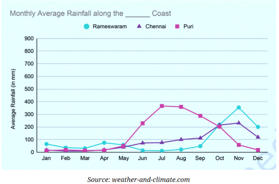
Solution:
The method to compile monthly average rainfall data involves:
- Data Collection: Rainfall is measured daily using rain gauges at meteorological stations in each city
- Monthly Totals: Daily rainfall measurements are added to get the total rainfall for each month
- Multi-year Recording: This process is repeated for several years (typically 30 years or more)
- Averaging: For each month (e.g., June), the total rainfall across all years is calculated and divided by the number of years
- Formula: Monthly Average Rainfall for June = (Sum of June rainfall for all years) {tex}\div{/tex} (Number of years]
This gives us the monthly average rainfall pattern for each city.
Q.44: Mark these cities on a map of India. What is common to how they are grouped in the graphs? Share your observations and inferences about the graphs.
Solution:
Geographical Grouping:
- West Coast cities: Kovalam (Kerala), Udupi (Karnataka), Mumbai (Maharashtra)
- East Coast cities: Rameswaram (Tamil Nadu), Chennai (Tamil Nadu), Puri (Odisha)
Common Observations:
- Cities are grouped by coastal location (east vs. west)
- West coast cities show similar rainfall patterns
- East coast cities show similar rainfall patterns
- West coast receives significantly more rainfall than east coast
- The timing of peak rainfall differs between the two coasts
Inferences:
- West coast cities receive heavy rainfall during June-August (South-West Monsoon)
- This is because monsoon winds from the Arabian Sea hit the Western Ghats
- East coast receives rainfall later in the year (October-December) from North-East Monsoon
- Geographical features like mountain ranges affect rainfall patterns
Q.45: Identify the peak months and low months of rainfall for each city.
Solution:
Peak Months:
- Udupl: June August (over 800 mm in July)
- Mumbal: June August (peak in July, around 800 mm )
- Kovalam: June August (peak in June, around 400 mm )
- Rameswaram: October December (peak in November, around 250 mm )
- Channel: October December (peak in November, around 350 mm )
- Purl: July September (peak in August, around 350 mm )
Low Months:
- All cities: January March are the driest months with minimal or no rainfall
- Special note for Rameswaram: Very Iow rainfall from January September (Iess than 50 mm )
Pattern Summary:
- West coast cities: Peak during South-West Monsoon (June-August)
- East coast cities: Peak during North-East Monsoon (October-December)
- Puri (though on east coast): Peak during South-West Monsoon like west coast cities
- Universal dry period: January March for all cities
Q.46: Read about the south-west monsoon and north-east monsoon and which regions come under the influence of these and when.
Solution:
South-West Monsoon (June September):
- Arrives from the Arabian Sea
- Affects entire India, especially west coast
- Brings heavy rainfall to Western Ghats
- Moisture-laden winds from the ocean hit the mountains causing orographic rainfall
- Responsible for 70-80% of India’s annual rainfall
- States most affected: Kerala, Karnataka, Maharashtra, Gujarat, and northeastern states
North-East Monsoon (October December):
- Also called “Retreating Monsoon” or “Winter Monsoon”
- Winds blow from land to sea, but pick up moisture over Bay of Bengal
- Primarily affects Tamil Nadu, coastal Andhra Pradesh, Karnataka, and Kerala
- Brings rain to southeastern coast
- Critical for Tamil Nadu’s agriculture
- Less intense than South-West Monsoon
This explains why Rameswaram and Chennai receive peak rainfall during October-December while Mumbai and Udupi receive it during June-August.
Q.47: The average number of customers visiting a shop and the average number of customers actually purchasing items over different days of the week is shown in the table below. Visualise this data on a line graph.
| Mon | Tue | Wed | Thu | Fri | Sat | Sun | |
| Visiting | 16 | 19 | 10 | 14 | 20 | 22 | 35 |
| Purchasing | 10 | 8 | 7 | 11 | 12 | 16 | 26 |
Solution:
To create the line graph:
Step 1: Set up axes
- X-axis: Days of the week (Mon to Sun)
- Y-axis: Number of customers (scale: 0 to 40, intervals of 5)
Step 2: Plot two lines
- Blue line for “Visiting” customers
- Red line for “Purchasing” customers
Step 3: Mark data points and connect
Observations from the graph:
- Sunday has the highest footfall (35 visitors, 26 purchases)
- Wednesday has the lowest footfall (10 visitors, 7 purchases)
- The gap between visiting and purchasing is largest on Tuesday (19-8 = 11)
- The conversion rate is highest on Thursday {tex}({1 1} / {1 4} \approx 79 \%){/tex}
- Weekend (Saturday and Sunday) shows significantly higher numbers
- The purchasing line always stays below the visiting line (as expected)
Q.48: The average number of days of rainfall in each month for a few cities is shown in the table below:
| Jan | Feb | Mar | Apr | May | Jun | Jul | Aug | Sep | Oct | Nov | Dec | |
| Mangaluru | 0.1 | 0 | 0.1 | 1.8 | 6.2 | 24.1 | 27.7 | 24.5 | 14 | 8.8 | 3.9 | 0.9 |
| New Delhi | ||||||||||||
| Port Blair | 2.4 | 1.3 | 0.9 | 3.3 | 15.5 | 18.7 | 17.3 | 18.8 | 16.8 | 14.1 | 11.3 | 5.4 |
| Rameswaram | 2.6 | 1.3 | 1.9 | 3.4 | 2.5 | 0.4 | 1 | 1 | 1.9 | 8.1 | 10.4 | 7.8 |
- What could be the possible method to compile this data?
- Mark the data for Mangaluru, Port Blair, and Rameswaram in the line graph shown below. You can round off the values to the nearest integer.
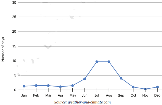
- Based on the line for New Delhi in the graph fill the data in the table.
- Which city among these receives the most number of days of rainfall per year? Which city gets the least number of days of rainfall per year?
- Looking at the table, when is the rainy season in New Delhi and Rameswaram?
Solution:
- The method to compile this data:
- Daily Recording: Meteorological departments record whether rainfall occurred each day (yes/no)
- Monthly Count: Count the total number of days with rainfall in each month
- Multi-Year Data: This is repeated for many years (typically 30+ years)
- Averaging: For each month, sum up the rainy days across all years and divide by the number of years
- Formula: Average rainy days in June {tex}={/tex} (Total rainy days in June across all years) ÷ (Number of years recorded)
- Rounding off to nearest integers:
Mangaluru: {tex}0,0,0,2,6,24,28,25,14,9,4,1{/tex}
Port Blair: 2, 1, 1, 3, 16, 19, 17, 19, 17, 14, 11, 5
Rameswaram: {tex}3,1,2,3,3,0,1,1,2,8,10,8{/tex}
Plotting Instructions:- Use different colors for each city
- Mark points at the rounded values for each month
- Connect consecutive points with straight lines
- Label each line with the city name
- Mangaluru shows a dramatic peak in June-July (24-28 days)
- Port Blair shows more consistent rainfall throughout the year
- Rameswaram shows peaks in October-November (8-10 days)
- Reading from the graph for New Delhi: Month Jan Feb Mar Apr May Jun Jul Aug Sep Oct Nov Dec New Delhi 2 2 3 2 3 4 8 8 4 1 1 2 The line for New Delhi shows relatively low rainfall days throughout the year, with a peak during the monsoon months (July-August) at approximately 8 days each.
- Let’s calculate the total rainy days per year for each city:
Mangaluru: {tex}0.1+0+0.1+1.8+6.2+24.1+27.7{/tex}{tex}+24.5+14+8.8+3.9+0.9={1 1 2 . 1}{/tex} days
New Delhi: {tex}2+2+3+2+3+4{/tex}{tex}+8+8+4+1+1+2=40{/tex} days
Port Blair: {tex}2.4+1.3+0.9+3.3+15.5+18.7+{/tex}17.3 + 18.8 + 16.8 + 14.1 + 11.3 + 5.4 = 125.8 days
Rameswaram: {tex}2.6+1.3+1.9+3.4+2.5+0.4{/tex}{tex}+1+1+1.9+8.1+10.4+7.8={4 2 . 3}{/tex} days
Answer:- Most rainy days: Port Blair with approximately {tex}{1 2 6}{/tex} days per year
- Least rainy days: New Delhi with approximately 40 days per year
New Delhi: - Rainy season: July August (monsoon months)
- Peak: 8 days of rainfall in both July and August
- Moderate rain: June and September (4 days each)
- This corresponds to the South-West Monsoon period
- Total monsoon contribution: June-September accounts for 24 out of 40 annual rainy days
- Rainy season: October December (North-East Monsoon)
- Peak: October ( 8.1 days), November ( 10.4 days), December ( 7.8 days)
- This period accounts for 26.3 days out of 42.3 total annual rainy days
- Very dry period: January September (only about 16 rainy days)
- This shows Rameswaram depends heavily on the North-East Monsoon
Comparison: New Delhi receives rain during South-West Monsoon (summer), while Rameswaram receives most rain during North-East Monsoon (winter), showing the regional variation in monsoon patterns across India.
Q.49: The following line graph shows the number of births in every month in India over a time period: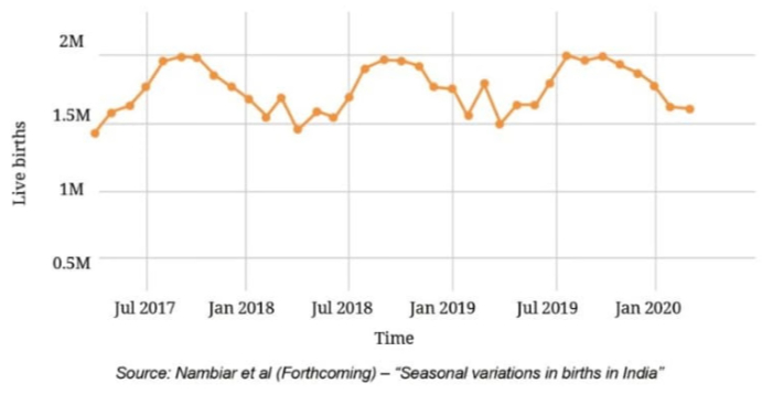
- What are your observations?
- What was the approximate number of births in July 2017?
- What time period does the graph capture?
- Compare the number of births in the month of January in the years 2018, 2019, and 2020.
- Estimate the number of births in the year 2019.
Solution:
- Key observations from the graph:Possible Reasons:
- Cyclical Pattern: There is a clear repeating annual pattern in the number of births
- Seasonal Variation: Births show seasonal peaks and troughs
- Peak Months: September-October typically show higher birth numbers (around 2.5 million per month)
- Low Months: April-May show lower birth numbers (around 2.0-2.1 million per month)
- Overall Trend: There’s a slight general increasing trend over the years
- Regular Fluctuations: The wave-like pattern repeats consistently each year
- Monthly Variation: Difference between peak and Iow months is approximately 400,000-500,000 births
- Predictability: The pattern is quite predictable and regular
- Peak births in September suggest conceptions in December-January (winter months)
- Cultural factors, festivals, and weather may influence conception patterns
- Agricultural cycles might play a role in rural areas
- Looking at the graph for July 2017 :
The graph shows that in July 2017, the number of births was approximately {tex}{2 . 3}{/tex} million or 23 lakh births.
This can be read by:- Locating July 2017 on the X-axis
- Following the vertical line up to meet the curve
- Reading the corresponding value on the {tex}Y{/tex}-axis
- The graph captures data from January 2016 to December 2020, approximately.
This is a period of 5 years or 60 months.
The X-axis shows years from 2016 to 2020, with monthly data points throughout this period. This allows us to observe birth patterns across multiple years and identify consistent seasonal trends.
Comparing January births across three years:
January 2018: Approximately 2.2 million (22lakh) births January 2019: Approximately
2.25 million (22.5 lakh) births January 2020: Approximately 2.3 million (23 lakh) births
Comparison:- Increasing Trend: There is a gradual increase in January births over these three years
- Rate of Increase:
- 2018 to 2019 : Increase of {tex}\sim 50,000{/tex} births ( {tex}2.3 \%{/tex} increase)
- 2019 to 2020 : Increase of {tex}\sim 50,000{/tex} births (2.2\% increase)
- Pattern: All three Januaries fall in the lower part of the annual cycle
- Consistency: The increase is steady and consistent
- Total Growth: From 2018 to 2020, January births increased by approximately 100,000(4.5\% growth over 2 years)
This reflects both population growth and consistent seasonal birth patterns.
- To estimate total births in 2019, we need to estimate births for each month and sum them:
Reading approximate values from the graph for 2019: MonthApproximate Births (in millions) January 2.25 February 2.15 March 2.10 April 2.05 May 2.00 June 2.10 July 2.30 August 2.40 September 2.50 October 2.50 November 2.35 December 2.30 Total births in {tex}2019=2.25+2.15+2.10+2.05+2.00{/tex}{tex}+2.10+2.30+2.40+2.50+2.50{/tex}{tex}+ 2.35+2.30={2 7 . 0}{/tex} million births {tex}={2 . 7}{/tex} crore births approximately
Alternative Method:- Average monthly births {tex}\approx 2.25{/tex} million
- Annual total {tex}=2.25 \times 12=27{/tex} million births
Therefore, approximately {tex}{2}{/tex} crore {tex}{7 0}{/tex} lakh babies were born in India in 2019.
Q.50: I wonder if there is anything common in all the states preferring rice or states preferring wheat.
Solution:
Yes, there are several common factors:
For Rice-Preferring States (Green regions):
- Geographical: Mostly coastal states and eastern India
- Climate: High rainfall, humid climate suitable for paddy cultivation
- Water Availability: Abundant water resources (rivers, monsoons)
- Agriculture: Traditional rice-growing regions with suitable soil
- Cultural: Rice deeply embedded in cultural practices and festivals
- Cuisine: Rice-based dishes dominate (idli, dosa, rice with curry)
- Historical: Long history of rice cultivation and consumption
For Wheat-Preferring States (Red regions):
- Geographical: Northern plains and central India
- Climate: Moderate rainfall, suitable for wheat cultivation
- Temperature: Cooler winters favorable for wheat
- Agriculture: Major wheat-producing regions
- Cultural: Wheat-based foods in traditions (roti, paratha)
- Cuisine: Bread-based meals dominate
- Historical: Indo-Gangetic plains known for wheat cultivation
Common Pattern: The red line dividing rice and wheat preferences roughly follows the Vindhya Range, showing how geography influences food culture!
Q.51: I want to know if the preferences were similar even 100 years ago.
Solution:
This is an excellent question for research!
Likely Scenario 100 Years Ago (1920s):
Similarities that probably existed:
- Regional patterns were likely similar due to:
- Climate and soil conditions haven’t changed drastically
- Traditional crops grown in suitable regions
- Cultural food habits passed through generations
- North-South divide probably existed
- Coastal areas likely preferred rice
- Punjab-Haryana region likely grew and consumed wheat
Possible Differences:
- Self-sufficiency: People consumed what grew locally
- Limited transport: Less mixing of food cultures
- Stronger regional preferences: Choices more rigid
- Green Revolution impact: Post-1960s, wheat production increased massively in Punjab-Haryana
- Urbanization: Modern cities show more mixed preferences
- PDS (Public Distribution System): Government distribution of rice/wheat has influenced consumption patterns
To find out:
- Study historical agricultural data
- Read about food habits in literature from that period
- Examine British colonial records on agriculture
- Interview elderly people about their grandparents’ food habits
- Research pre-Green Revolution food patterns
This would make an excellent research project!
Q.52: Mean Grids: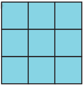
- Fill the grid with 9 distinct numbers such that the average along each row, column, and diagonal is 10.
- Can we fill the grid by changing a few numbers and still get 10 as the average in all directions?
Solution:
- 16 2 12 6 10 14 8 18 4 Verification:
- Each row, column, and diagonal sums to 30
- Average {tex}=30 / 3=10{/tex}
- All 9 numbers are distinct
- Yes! There are multiple solutions.
Method 1: Use transformations|f we have one solution, we can create others by:- Adding the same number to all elements (changes average)
- Reflecting the grid (swapping rows or columns)
- Rotating the grid
Alternative Solution: 1 18 11 16 10 4 13 2 15
Key Point: There are exactly 8 variations of the basic magic square {tex}(3 \times 3){/tex} centered at 10 :
- 1 original
- 3 rotations {tex}\left(90^{\circ}, 180^{\circ}, 270^{\circ}\right){/tex}
- 4 reflections
All will satisfy the condition of averaging to 10 in all directions!
Q.53: Give two examples of data that satisfy 3 numbers whose mean is 8.
Solution:
Method: Mean {tex}=({/tex}Sum of all numbers{tex}) \div({/tex}Count of numbers{tex}){/tex}
If mean {tex}=8{/tex} and count {tex}=3{/tex}, then Sum {tex}=8 \times 3=24{/tex}
Example 1: 6, 8, 10
- Sum {tex}=6+8+10=24{/tex}
- Mean {tex}=24 \div 3=8{/tex}
Example 2: 2, 10, 12
- Sum {tex}=2+10+12=24{/tex}
- Mean {tex}=24 \div 3=8{/tex}
Other possibilities: {tex}0,8,16{/tex} or {tex}1,7,16{/tex} or {tex}5,9,10{/tex}, etc.
Q.54: Give two examples of data that satisfy 4 numbers whose median is 15.5.
Solution:
Method: For 4 numbers, median = Average of 2nd and 3rd numbers {tex}({/tex}when arranged in order)
If median {tex}=15.5{/tex}, then {tex}(2{/tex}nd number + 3rd number{tex}) \div 2=15.5{/tex}
Therefore, 2nd number + 3rd number {tex}=31{/tex}
Example 1: {tex}10,15,16,20{/tex}
- Arranged: {tex}10,15,16,20{/tex}
- Median {tex}=(15+16) \div 2=31 \div 2=15.5{/tex}
Example 2: 5, 14, 17, 25
- Arranged: {tex}5,14,17,25{/tex}
- Median {tex}=(14+17) \div 2=31 \div 2=15.5{/tex}
Other possibilities: {tex}1,10,21,100{/tex} or {tex}8,13,18,30{/tex}, etc.
Q.55: Give two examples of data that satisfy 5 numbers whose mean is 13.6.
Solution:
Method: If mean {tex}=13.6{/tex} and count {tex}=5{/tex}, then Sum {tex}=13.6 \times 5=68{/tex}
Example 1: 10, 12, 14, 15, 17
- Sum {tex}=10+12+14+15+17=68{/tex}
- Mean {tex}=68 \div 5=13.6{/tex}
Example 2: 5, 10, 15, 18, 20
- Sum {tex}=5+10+15+18+20=68{/tex}
- Mean {tex}=68 \div 5=13.6{/tex}
Other possibilities: {tex}13,13,13,14,15{/tex} or {tex}1,10,20,21,16{/tex}, etc.
Q.56: Give two examples of data that satisfy 6 numbers whose mean = median.
Solution:
Method: For 6 numbers, median {tex}={/tex} Average of 3rd and 4th numbers
We need: Mean = Median
Example 1: 1, 2, 3, 4, 5, 6
- Mean {tex}=(1+2+3+4+5+6) \div 6=21 \div 6=3.5{/tex}
- Median {tex}=(3+4) \div 2=7 \div 2=3.5{/tex}
- Mean {tex}={/tex} Median
Example 2: 5, 10, 15, 15, 20, 25
- Mean {tex}=(5+10+15+15+20+25) \div 6=90 \div 6=15{/tex}
- Median {tex}=(15+15) \div 2=30 \div 2=15{/tex}
- Mean {tex}={/tex} Median
Note: Symmetric distributions often have mean {tex}={/tex} median!
Q.57: Give two examples of data that satisfy 6 numbers whose mean > median.
Solution:
Method: Mean>Median happens when there are large values pulling the average up This occurs in right-skewed distributions
Example 1: 1,2,3,4,5,15
- Mean {tex}=(1+2+3+4+5+15) \div 6=30 \div 6=5{/tex}
- Median {tex}=(3+4) \div 2=7 \div 2=3.5{/tex}
- Mean (5) > Median (3.5)
Example 2: 2, 4, 6, 8, 10, 30
- Mean {tex}=(2+4+6+8+10+30) \div 6=60 \div 6=10{/tex}
- Median {tex}=(6+8) \div 2=14 \div 2=7{/tex}
- Mean (10) > Median (7)
Q.58: Fill in the blanks such that the median of the collection is {tex}13: 5,21{/tex}, 14, ________, ________, ________. How many possibilities exist if only counting numbers are allowed?
Solution:
Analysis:
- We have 6 numbers total: {tex}5,21,14{/tex}, ________, ________, ________
- For 6 numbers, median {tex}={/tex} average of 3rd and 4th numbers (when arranged)
- Required median {tex}=13{/tex}
Step 1: Arrange given numbers: {tex}5,14,21{/tex}
Step 2: For median {tex}=13{/tex}, we need {tex}(3 {rd}{/tex} number +4th number {tex}) \div 2=13{/tex}
Therefore, 3rd number + 4th number {tex}=26{/tex}
Possibilities:
Case 1: Both blanks are less than or equal to 14
Then arranged: 5, ________, ________14, 21, ________
For median to be 13: middle two must be such that their average is 13 Not possible as {tex}14>13{/tex}
Case 2: One blank less than 5, others between 5 and 21
Example: {tex}3,5,12,14,15,21{/tex}
Median {tex}=(12+14) / 2=13{/tex}
Case 3: Blanks are strategically placed the 3rd and 4th positions (when arranged) must. average to 13
Systematic Solution:
Let the three blanks be a, b, c
Configuration 1: {tex}a, b, c{/tex} all between 5 and 21
Arranged: 5, a, b, c, 14, 21 (if a, b, c<14)
We need {tex}b+c=26{/tex}
- Possibilities: (12,14) already used, (11,15), (10,16), (9,17), (8,18), (7,19), (6,20), etc.
Wait, we need to be more careful about arrangement.
Better Approach:
Given: {tex}5,14,21{/tex}, andthree unknowns a, b, c
Arranged in order, for median {tex}=13{/tex},the 3rd and 4th values must average to 13.
Possible scenarios:
If arranged as: {tex}5, a, b, c, 14,21{/tex}then {tex}b+c=26{/tex}, where {tex}a<b<c<14{/tex}
Example 1: {tex}{a}=6, {~b}=12, {c}=14{/tex} (but 14 already used)
Let’s say {tex}{a}=6, {~b}=11, {c}=15{/tex}
Check: 5,6, {tex}11,14,15,21{/tex} Median {tex}=(11+14) / 2=25 / 2=12.5 \neq 13{/tex}
Correct thinking: For 3rd + 4th = 26:
- If 14 is 4th,then {tex}3 {rd}=12{/tex}: Arranged: {tex}5, {a}, 12,14, {~b}, 21{/tex}
- If 14 is 5th or later, then we need two numbers that sum to 26
Valid Example 1: {tex}5,10,12,14,16,21{/tex}
Median {tex}=(12+14) / 2=13{/tex}
Blanks: {tex}10,12,16{/tex}
Valid Example 2: {tex}5,11,13,14,15,21{/tex}
Median {tex}=(13+14) / 2=13.5 \neq 13{/tex}
Valid Example {tex}2({/tex}corrected{tex}): 5,9,12,14,17,21{/tex}
Median {tex}=(12+14) / 2=13{/tex} Blanks: 9,12, 17
How many possibilities?
For counting numbers:
- 3rd position can be: {tex}6,7,8,9,10,11,12,13{/tex} (lessthan 14 )
- 4th position is 14 (fixed)
- For each, calculate 4th needed to sum to 26
Actually, let’sthink differently:
- If 3rd is 12 and 4th is 14: median {tex}=13{/tex}
- We need exactly one number to be 12, one to be 14, and remaining can be anything
Since 14 is already inthe list, we need to add 12 and one more number (can be anything)
Answer: Infinite possibilities if we only need median {tex}=13!{/tex}
We can have any combination where:
- One blank {tex}=12{/tex}
- Other two blanks can be ANY counting numbers
- As long as when arranged, 12 and 14 are in 3rd and 4th positions
Examples:
- {tex}(1,12,100) \rightarrow{/tex} Arranged: {tex}1,5,12,14,21,100 \rightarrow{/tex} Median {tex}=13{/tex}
- {tex}(2,12,50) \rightarrow{/tex} Arranged: {tex}2,5,12,14,21,50 \rightarrow{/tex} Median {tex}=13{/tex}
- {tex}(12,15,20) \rightarrow{/tex} Arranged: {tex}5,12,14,15,20,21 \rightarrow{/tex} Median {tex}=(14+15) / 2=14.5{/tex}
Wait,the position of 14 changes!
Correct Analysis:
For median {tex}=13{/tex} with 6 numbers, we need {tex}3 {rd}+4 {th}=26{/tex}
Given: 5, 14, 21
Scenario 1: 14 is in 4th position then 3rd must be 12
Need: One value {tex}\leq 5{/tex}, one value {tex}=12{/tex}, one value between 14 and 21
Example: {tex}3,5,12,14,18,21 \rightarrow{/tex} Median {tex}=13{/tex}
Scenario 2: 14 is in 5th or 6th position then 3rd and 4th are both new numbers summing to 26
After careful analysis: Infinite possibilities exist!
Q.59: Fill in the blanks such that the mean of the collection is {tex}6.5: 3,11{/tex}, ________, ________, 15, 6. How many possibilities exist if only counting numbers are allowed?
Solution:
Given numbers: 3, 11, ________, ________, 15, 6
Total numbers {tex}=6{/tex}
Mean {tex}=6.5{/tex}
Sum of all 6 numbers {tex}={/tex} Mean {tex}\times{/tex} Number of values {tex}=6.5 \times 6=39{/tex}
Sum of known numbers {tex}=3+11+15+6=35{/tex}
Sum of two unknown numbers {tex}=39-35=4{/tex}
We need two counting numbers that sum to 4 :
- {tex}1+3=4{/tex}
- {tex}2+2=4{/tex}
- {tex}0+4=4{/tex} (if O is considered a counting number)
Solution 1: 3, 11, 1, 3, 15, 6
- Sum {tex}=3+11+1+3+15+6=39{/tex}
- Mean {tex}=39 \div 6=6.5{/tex}
Solution 2: 3, 11, 2, 2, 15, 6
- Sum {tex}=3+11+2+2+15+6=39{/tex}
- Mean {tex}=39 \div 6=6.5{/tex}
How many possibilities? |f only counting numbers (natural numbers: {tex}1,2,3, \ldots{/tex}) are allowed:
- (1,3) and (3,1) – same pair, different order
- {tex}(2,2){/tex} only one way
If we consider order:
- 3 possibilities: {tex}(1,3),(3,1),(2,2){/tex}
If we don’t consider order:
- 2 possibilities: {tex}\{1,3\}{/tex} and {tex}\{2,2\}{/tex}
Q.60: Check whether each of the statements below is true. Justify your reasoning. Use algebra, if necessary, to justify.
- The average of two even numbers is even.
- The average of any two multiples of 5 will be a multiple of 5.
- The average of any 5 multiples of 5 will also be a multiple of 5.
Solution:
- Algebraic proof: Let the two even numbers be {tex}2 m{/tex} and {tex}2 n{/tex} (where {tex}m{/tex} and {tex}n{/tex} are whole numbers).
Average {tex}=(2 m+2 n) \div 2=2(m+n) \div 2=m+n{/tex}
Since {tex}m{/tex} and {tex}n{/tex} are whole numbers, {tex}(m+n){/tex} is also a whole number.
Wait, this shows the average is a whole number, not necessarily even!
Let’s reconsider: Average {tex}=(2 m+2 n) \div 2=(m+n){/tex}
If {tex}{m}+{n}{/tex} is even, then average is even. If {tex}{m}+{n}{/tex} is odd, then average is odd.
Counter- example:- Numbers: 2 and 4 (both even)
- Average {tex}=(2+4) \div 2=3{/tex} (odd!)
Correct statement: The average of two even numbers is a whole number, but not necessarily even. - Not always TRUE
Algebraic approach:Let the two multiples of 5 be {tex}5 m{/tex} and {tex}5 n{/tex} (where {tex}m{/tex} and {tex}n{/tex} are whole numbers).
Average {tex}=(5 m+5 n) \div 2=5(m+n) \div 2{/tex}
For this to be a multiple of 5 , we need {tex}(m+n) \div 2{/tex} to be a whole number.
This is true only when {tex}(m+n){/tex} is even.
Counter-example:- Numbers: 5 and 10 (both multiples of 5)
- Average {tex}=(5+10) \div 2=15 \div 2=7.5{/tex} (NOT a multiple of 5)
- Numbers: 10 and 20 (both multiples of 5)
- Average {tex}=(10+20) \div 2=30 \div 2=15{/tex} (multiple of 5)
- TRUE
Algebralc proof: Let the five multiples of 5 be 5a, 5b, 5c, 5d, and 5e (where {tex}a, b, c, d{/tex}, e are whole numbers].
Average {tex}=(5 a+5 b+5 c+5 d+5 e) \div{/tex}{tex} 5=5(a+b+c+d+e) \div 5=a+b+c+d+e{/tex}
Since {tex}a, b, c, d, e{/tex} are whole numbers, their sum ( {tex}a+b+c+d+e{/tex} ) is also a whole number.
But walt, we need to show It’s a multiple of 5!
Let me reconsider: Sum {tex}=5 a+5 b+5 c+5 d+5 e=5(a+b+c+d+e){/tex}
Average {tex}=5(a+b+c+d+e) \div 5=(a+b+c+d+e){/tex}
This is a whole number but not necessarily a multiple of 5.
Counter-example:- Numbers: 5, 5, 5, 5, 5 (all multiples of 5)
- Sum {tex}=25{/tex}
- Average {tex}=25 \div 5=5{/tex} (multiple of 5)
- Numbers: 5, 10, 15, 20, 25 (all multiples of 5)
- Sum {tex}=75{/tex}
- Average {tex}=75 \div 5=15{/tex} (multiple of 5)
This sum is always a multiple of 5.
When we divide by {tex}5: 5(a+b+c+d+e){/tex}{tex} \div 5=(a+b+c+d+e){/tex}
Hmm, this gives a whole number, not necessarily a multiple of 5 .
Let me reconsider the question interpretation:
Actually, the sum of 5 multiples of 5 is definitely a multiple of 5. When we divide this sum by 5, we get a whole number.
But the question asks if the AVERAGE is a multiple of 5.
Counter-example:- Numbers: 5, 5, 5, 5, 10
- Sum {tex}=30{/tex}
- Average {tex}=30 \div 5=6{/tex} (NOT a multiple of 5)
Q.61: There were 2 new admissions to Sudhakar’s class just a couple of days after the class average height was found to be 150.2 cm. Which of the following statements are correct? Why?
Options:
(1)
The average height of the class will increase as there are 2 new values.
(2)
The average height of the class will remain the same.
(3)
The heights of the new students have to be measured to find out the new average height. ✅
(4)
The heights of everyone in the class has to be measured again to calculate the new average height.
Explanation:
We must know the heights of the new students to calculate the new average. Without this information, we cannot determine how the average will change.
Q.62: There were 2 new admissions to Sudhakar’s class just a couple of days after the class average height was found to be 150.2 cm. The heights of the two new joinees are 149 cm and 152 cm. Which of the following statements about the class average height are correct? Why?
Options:
(1) The average will remain the same.
(2) The average will increase. ✅
(3) The average will decrease.
(4) The information is not sufficient to make a claim about the average.
Explanation:
The average of the two new students ({tex}{1 5 0 . 5 ~ c m}{/tex}) is greater than the current class average (150.2 cm). When we add students whose average is higher than the current average, the overall average increases.
Mathematical verification: Let’s say there were originally 20 students.
- Original total height {tex}=150.2 \times 20=3004 {~cm}{/tex}
- New total height {tex}=3004+149+152=3305 {~cm}{/tex}
- New average {tex}=3305 \div 22=150.227 \ldots {~cm}>150.2 {~cm}{/tex}
Q.63: There were 2 new admissions to Sudhakar’s class just a couple of days after the class average height was found to be 150.2 cm. Which of the following statements about the new class average height are correct? Why?
Options:
(1) The median will remain the same.
(2) The median will increase.
(3) The median will decrease.
(4) The information is not sufficient to make a claim about median. ✅
Explanation: To determine the median:
- We need to know all individual heights
- We need to arrange them in order
- We need to find the middle value
- Just knowing the average and two new values is not enough
Example showing why:
- If the class has 10 students with heights: 140, 145, 148, 150, 151, 151, 152, 153, 155, 160
- Median {tex}=(151+151) \div 2=151 {~cm}{/tex}
- Adding 149 and 152: 140, 145, 148, 149, 150, 151, 151, 152, 152, 153, 155, 160
- New median {tex}=(151+151) \div 2=151 {~cm}{/tex} (remained same)
In another distribution, the median might change.
Q.64: Is 17 the average of the data shown in the dot plot below? Share the method you used to answer this question.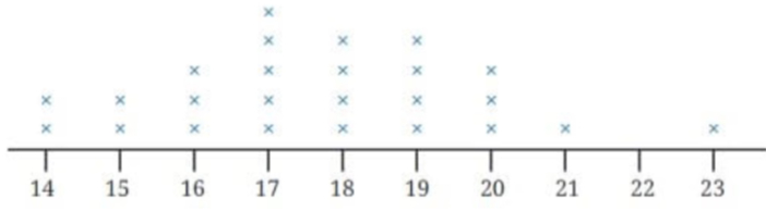
[Dot plot showing data points from 14 to 23]
Solution:
Method 1: Count and Calculate
From the dot plot, let’s count the frequency of each value:
- 14: 2 dots
- 15:3 dots
- 16:4 dots
- 17:3 dots
- 18: 2 dots
- 19:3 dots
- 20: 2 dots
- 21: 2 dots
- 22: 1 dot
- 23: 2 dots
Total number of data points {tex}=2+3+4+3+2{/tex}{tex}+3+2+2+1+2=24{/tex}
Sum of all values: {tex}=(14 \times 2)+(15 \times 3)+(16 \times 4)+{/tex}{tex}(17 \times 3)+(18 \times 2)+(19 \times 3)+(20 \times 2)+{/tex} {tex} (21 \times 2)+(22 \times 1)+(23 \times 2){/tex} {tex}=28+45+64+51+36{/tex}{tex}+57+40+42+22+46=431 {/tex}
Average {tex}=431 \div 24=17.958 \ldots \approx 18{/tex}
Answer: No, 17 is NOT the average. The average is approximately 18.
Method 2: Visual Balance Method
We can observe that:
- There are more dots on the right side of 17 (at 18, 19, 20, 21, 22, 23)
- The values on the right are farther from 17 than most values on the left
- This suggests the average is pulled slightly to the right of 1
Conclusion: The average is greater than 17, approximately 18.
Q.65: The weights of people in a group were measured every month. The average weight for the previous month was 65.3 kg and the median weight was 67 kg. The data for this month showed that one person has lost 2 kg and two have gained 1 kg. What can we say about the change in mean weight and median weight this month?
Solution:
Change in Mean Weight:
Let’s say there are n people in the group.
Previous month:
- Total weight {tex}=65.3 \times {nkg}{/tex}
This month:
- One person lost 2 kg: -2 kg
- Two people gained 1 kg each: {tex}+1+1=+2 {~kg}{/tex}
- Net change {tex}=-2+2=0 {~kg}{/tex}
New total weight {tex}=65.3 \times {n}+0=65.3 \times {nkg}{/tex}
New mean {tex}=65.3 \times {n} \div {n}=65.3 {~kg}{/tex}
Conclusion about mean: The mean weight will REMAIN THE SAME ({tex}{6 5 . 3 ~ k g}{/tex}) because the total weight hasn’t changed.
Change in Median Weight:
The median depends on the middle value(s) when weights are arranged in order.
Previous month median {tex}=67 {~kg}{/tex}
What happens this month?
- One person’s weight decreased by 2 kg
- Two people’s weights increased by 1 kg each
Effect on median:
- If the person who lost weight was below or at the median, their new weight might still be below the median {tex}\rightarrow{/tex} median might stay same or decrease
- If the people who gained weight were above or at the median, their new weights might still be above the median {tex}\rightarrow{/tex} median might stay same or increase
- Without knowing the exact distribution and who changed weight, we cannot determine the exact change
Possible scenarios:
- If the person who lost 2 kg had weight {tex}<67 {~kg}{/tex}, and the two who gained 1 kg each had weights > 67 kg:
- The median might remain 67 kg
- If the person who lost 2 kg had weight exactly 67 kg (was at median):
- The median might decrease
- If the two people who gained {tex}{1} {~ k g}{/tex} were below median and moved closer to or above median:
- The median might increase or stay same
Conclusion about median: We CANNOT determine the exact change in median without knowing:
- The complete distribution of weights
- Which specific individuals changed weight
- How many people are in the group
Summary:
- Mean: Will remain the same (65.3 kg)
- Median: Cannot be determined without more information
Q.66: The following table shows the retail price (in ₹) of iodised salt in the month of January in a few states over 10 years. For your calculations and plotting you may round off values to the nearest counting number.
| Andaman and Nicobar Islands | Assam | Gujarat | Mizoram | Uttar Pradesh | West Bengal | |
| 2016 | 16 | 6 | 16.5 | 20 | 16.15 | 9.47 |
| 2017 | 12 | 12 | 14.75 | 20 | 16.97 | 11.65 |
| 2018 | 12 | 12 | 14.75 | 22 | 16.18 | 11.63 |
| 2019 | 12 | 12 | 14.75 | 22 | 18.24 | 11.43 |
| 2020 | 13.88 | 12 | 13 | 20 | 18.96 | 11.11 |
| 2021 | 18.22 | 15 | 14.45 | 22 | 20.63 | 12.79 |
| 2022 | 18.73 | 14 | 14.28 | 25 | 21.3 | 16.14 |
| 2023 | 20.63 | 12.02 | 14.54 | 27.65 | 25.39 | 18.43 |
| 2024 | 19.73 | 13.72 | 14.8 | 29.03 | 26.9 | 21.66 |
| 2025 | 20.99 | 12.35 | 19.2 | 29.8 | 24.81 | 23.99 |
- Choose data from any 3 states you find interesting and present it through a line graph using an appropriate scale.
- What do you find interesting in this data? Share your observations.
- Compare the price variation in Gujarat and Uttar Pradesh.
- In which state has the price increased the most from 2016 to 2025?
- What are you curious to explore further?
Solution:
- Let’s choose Gujarat, Mizoram, and West Bengal as these show interesting patterns.
Rounded data: YearGujaratMizoramWest Bengal 2016 17 20 9 2017 15 20 12 2018 15 22 12 2019 15 22 11 2020 13 20 11 2021 14 22 13 2022 14 25 16 2023 15 28 18 2024 15 29 22 2025 19 30 24 Line Graph:[Students should draw a line graph with:- X-axis: Years (2016 to 2025)
- Y-axis: Price in ₹ (scale: 0 to 35, with intervals of 5)
- Three different colored lines for the three states
- Legend indicating which line represents which state]
- Interesting observations:
- Gujarat shows remarkable price stability:
- Price remained around ₹13-17 from 2016 to 2024
- Only a significant jump to ₹19in 2025
- Most stable prices among all states
- Mizoram shows consistent upward trend:
- Started at ₹20 in 2016
- Reached ₹30 in 2025
- Increase of ₹10(50% increase)
- Most expensive salt throughout the period
- West Bengal shows dramatic increase:
- Started at ₹9 in 2016 (cheapest)
- Reached ₹24 in 2025
- Increase of ₹15 (about 167% increase!)
- Steepest increase especially after 2021
- General trend:
- Most states show price increases from 2021 onwards
- This could be related to inflation, COVID-19 pandemic effects, or supply chain issues
- Price range across states:
- In 2016: ₹6 (Assam) to ₹20 (Mizoram) large variation
- In 2025: ₹ 12 (Assam) to ₹30 (Mizoram) still large variation
- Gujarat:
- 2016: ₹17(rounded from 16.5)
- 2025: ₹19
- Change: ₹2 increase
- Percentage increase: {tex}(2 \div 17) \times 100 \approx 11.8 \%{/tex}
- Pattern: Very stable, minimal variation year to year
- Uttar Pradesh:
- 2016: ₹16
- 2025: ₹25 (rounded from 24.81)
- Change: ₹9increase
- Percentage increase: {tex}(9 \div 16) \times 100 \approx 56.25 \%{/tex}
- Pattern: Steady increase, especially after 2020
- Gujarat shows remarkable price stability:
- Let’s calculate the price increase for all states: State2016 Price2025 PriceIncrease (₹)% Increase Andaman & Nicobar ₹16 ₹21 ₹5 31.25% Assam ₹6 ₹12 ₹6 100% Gujarat ₹17 ₹19 き2 11.76% Mizoram ₹20 き30 ₹10 50% Uttar Pradesh ₹16 ₹25 ₹9 56.25% West Bengal ₹9 ₹24 ₹15 166.67% In absolute terms (₹):West Bengal has the highest increase of ₹15
In percentage terms: West Bengal also has the highest increase of 166.67%
Analysis:- West Bengal started with the second-lowest price (₹9)
- By 2025, it reached ₹24
- This is an increase of about {tex}167 \%{/tex}
- The price has more than doubled!
- Even Assam, which had {tex}100 \%{/tex} increase (doubled), increased by only ₹ 6 in absolute terms
Answer: West Bengal has seen the maximum price increase, both in absolute terms (₹15) and percentage terms (167%).
- Some interesting questions to explore:
- Why such large variation between states?
- Is it due to transportation costs?
- Different state taxes or subsidies?
- Local production vs. imports?
- Why did West Bengal’s price increase so dramatically?
- Was there a change in state policy?
- Supply chain disruptions?
- Increased demand?
- How does salt price compare to general inflation?
- Is salt price increase higher or lower than overall inflation?
- What other essential commodities followed similar patterns?
- Why is Mizoram consistently the most expensive?
- Is it due to transportation to remote areas?
- Limited local production?
- Higher demand?
- Why is Gujarat’s price so stable?
- Government price controls?
- Large local production (Gujarat has coastal areas)?
- Effective supply chain management?
- Impact of COVID-19 pandemic:
- Did prices spike during 2020-2021 due to supply disruptions?
- How quickly did they recover?
- Regional patterns:
- Do coastal states have cheaper salt?
- Do landlocked or hilly states have more expensive salt?
- Quality differences:
- Are the price differences also due to quality variations?
- Different types of iodised salt?
- Why such large variation between states?
Q.67: Referring to the graph below, which of the following statements are valid? Why?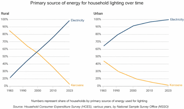
- In 1983, the majority in rural areas used kerosene as a primary lighting source while the majority in urban areas used electricity.
- The use of kerosene as a primary lighting source has decreased over time in both rural and urban areas.
- In the year 2000, 10% of the urban households used electricity as a primary lighting source.
- In 2023, there were no power cuts.
Solution:
- TRUE
From the graph:- Rural areas in 1983: The kerosene line is above {tex}50 \%{/tex} mark, while electricity line is below 50%
- Urban areas in 1983: The electricity line is well above {tex}50 \%{/tex} (appears to be around 70-80%), while kerosene is below 50%
- .”Majority” means more than {tex}50 \%{/tex}
- In rural areas, more than {tex}50 \%{/tex} used kerosene
- In urban areas, more than {tex}50 \%{/tex} used electricity
- Therefore, the statement is valid
- TRUE
From the graph:- Rural areas: The kerosene line (dashed) shows a steady decline from 1981 to 2023, going from around 80-90% to nearly 0%
- Urban areas: The kerosene line shows a decline from around {tex}30-40 \%{/tex} in 1981 to nearly 0% by 2023
- Both lines show downward trends
- This indicates decreased usage of kerosene
- Correspondingly, electricity usage increased
- This reflects rural electrification and development
Therefore, the statement is valid
- FALSE
From the graph:- In 2000 , the electricity line for urban areas is very high, around {tex}90-95 \%{/tex}
- This means about {tex}90-95 \%{/tex} of urban households used electricity
- NOT 10%
The statement says “10% used electricity” which is incorrect.
Possible confusion: Perhaps it means “10% used kerosene” or “90% used electricity”
Therefore, the statement is NOT valid
- FALSE/CANNOT BE DETERMINED
The graph shows:- In 2023 , nearly {tex}100 \%{/tex} of both rural and urban households used electricity as the primary lighting source
- Kerosene usage is nearly 0%
However:- The graph shows what people use as their “primary” lighting source
- It does NOT provide information about power cuts or electricity availability
- Even if electricity is the primary source, there could still be power cuts
- During power cuts, people might use other sources temporarily
- Primary lighting source means what they mainly rely on
- It doesn’t mean electricity is available 24/7 without interruptions
- The graph cannot tell us about power cuts
Therefore, the statement CANNOT BE VALIDATED from this graph. It’s an invalid conclusion
Q.68:
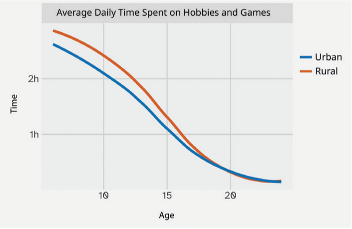
How long do children aged 10 in urban areas spend each day on hobbies and games?
Solution:
From the line graph:
- Look at age 10 on the x-axis
- Find the urban line (one of the two lines shown)
- Read the corresponding value on the y-axis (time in hours)
Answer: Children aged 10 in urban areas spend approximately 1.5 hours per day on hobbies and games.
Q.69:
At what age is the average time spent daily on hobbies and games by rural kids 1.5 hours?
- 8 years
- 10 years
- 12 years
- 14 years
- 18 years
Solution:
From the line graph:
- Find the rural line (one of the two lines)
- Locate where this line crosses the 1.5 hours mark on the $y$-axis
- Read the corresponding age on the $x$-axis
Answer: (c) 12 years
At age 12 , rural children spend approximately 1.5 hours per day on hobbies and games.
Q.70:
Are the following statements correct?
- The average time spent daily on hobbies and games by kids aged 15 is twice that of kids aged 10.
- All rural kids aged 15 spend at least 1 hour on hobbies and games everyday.
Solution:
- To verify this:
- Find time spent by 10 -year-olds (both rural and urban)
- Find time spent by 15 -year-olds (both rural and urban)
- Check if time at age {tex}15=2 \times{/tex} time at age 10
Approximate values from typical such graphs: - Urban kids aged 10: {tex}\sim{/tex}1.5 hours
- Urban kids aged 15: {tex}\sim{/tex}1 hour (Actually decreases!)
- Rural kids aged 10: {tex}\sim{/tex}2hours
- Rural kids aged 15: {tex}\sim{/tex}1.5 hours (Also decreases!)
Answer: FALSE
- Time spent on hobbies and games typically DECREASES as children grow older (more academic pressure, entrance exams, etc.)
- At age 15, children spend LESS time, not double, compared to age 10
- Answer: FALSE
Why this statement is incorrect:- The graph shows AVERAGE time:
- The line represents the average (mean) time spent
- It does NOT show individual data points
- Average doesn’t mean “all”:
- If average is 1.5 hours, some children might spend 0 hours, some might spend 3 hours
- The average being above 1 hour doesn’t mean ALL children spend at least 1 hour
- Example to illustrate:
- If 10 children have times: {tex}0,0.5,1,1,1.5,1.5,2,2,2.5,3{/tex} hours
- Average {tex}=15 \div 10=1.5{/tex} hours
- But 2 children spend LESS than 1 hour
Conclusion: We cannot make statements about “all” individuals based on average data. The statement is NOT correct.
- The graph shows AVERAGE time:
Q.71: Individual project: Make your own activity strip for different days of the week.
- Do you eat and sleep at regular times every day? Typically how long do you spend outdoors?
- Calculate the average time spent per activity. Represent this average day using a strip.
- Similarly, track the activities of any adult at home. Compare your data with theirs.
Solution:
- This is a personal reflection question. Here’s a sample response:
My Daily Routine Analysis:
Eating Times:- Breakfast: Usually between 7:00-7:30 AM (fairly regular on school days)
- Lunch: 1:00-1:30 PM on school days; 2:00-2:30 PM on weekends (somewhat irregular)
- Dinner: 8:00-8:30 PM (mostly regular)
- Weekdays: Sleep by 10:00 PM, wake up at 6:00 AM (8 hours)
- Weekends: Sleep by 11:00 PM, wake up at 8:00 AM (9 hours)
- Weekdays: About 1 hour (traveling to school + playing)
- Weekends: About 2-3 hours (playing with friends, going to park)
- Meal times are fairly regular on weekdays but less regular on weekends
- Sleep schedule shifts by about 1-2 hours on weekends
- I spend more time outdoors on weekends
[Students should write their own observations based on their actual routines]
- Sample Calculation for a week:
Let’s track activities for 7 days and find averages:
Activities tracked:- Sleeping
- School/Study
- Eating
- Playing/Hobbies
- Screen time (TV/Mobile)
- Personal care
- Other activities
- Sleep: {tex}(8+8+7.5+8+8+9+9) \div 7=57.5 \div 7 \approx 8.2{/tex} hours
- School/Study: {tex}(8+8+8+8+7+4+3) \div 7=46 \div 7 \approx 6.6{/tex} hours
- Eating: {tex}(2+2+2+2+2+2+2.5) \div 7=14.5 \div 7 \approx 2.1{/tex} hours
- Playing: {tex}(1+1.5+1+1+2+3+3) \div 7=12.5 \div 7 \approx 1.8{/tex} hours
- Screen time: {tex}(2+1.5+2+2+2+3+3) \div 7=15.5 \div 7 \approx 2.2{/tex} hours
- Personal care: {tex}(2+2+2+2+2+2+2) \div 7=14 \div 7=2{/tex} hours
- Other: {tex}(1+1+1.5+1+1+1+1.5) \div 7=8 \div 7 \approx 1.1{/tex} hours
|–Sleep (8.2h)–|–School/Study (6.6h)–|–Screen (2.2h)–|–Eating (2.1h)–|–Playing (1.8h
[Color code each segment and label with hours] - Sample: Tracking Mother’s Activities
Average day for mother:- Sleep: 7 hours
- Work (job/housework): 10 hours
- Eating: 2 hours
- Recreation: 1 hour
- Personal care: 2 hours
- Other: 2 hours
- Mother sleeps less than me
- Mother works significantly more hours (includes job + housework)
- I have more free time for playing and screen time
- Adults have more responsibilities and less leisure time
- Both of us spend similar time on eating and personal care
- As a student, my main “work” is school and study
- Adults have longer working hours
- Adults sacrifice sleep and recreation time for responsibilities
- Children have more time for hobbies and play
[Students should do this activity with their own family members and make genuine observations]
Q.72: Small group project: Make a group of {tex}3-4{/tex} members. Do at least one of the following:
- Track daily sleep time of all your family members for a week. Daily sleep time includes night sleep, naps, and any sleep during the day.
- Represent this on strips.
- Put together the data of all your group members. Calculate the average and median sleep time of children, adults, elderly.
- Share your findings and observations.
- When do schools start and end? On a weekday, Manoj’s school starts at 9:30 am and ends at 4:30 pm, i.e., 7 hours which include class time and breaks. Collect information on the daily timings of different schools for Grade 8, including class time and break time (the schools can be anywhere in the country. You can ask your neighbours, relatives, parents and friends to find out). Analyse and present the data collected.
Solution:
Do it yourself.
Q.73: The following graphs show the sunrise and sunset times across the year at 4 locations in India. Observe how the graphs are organised. Are you able to identify which lines indicate the sunrise and which indicate the sunset?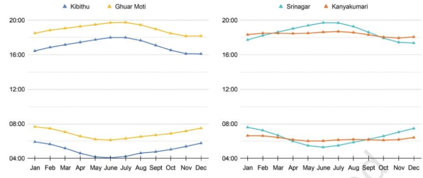
Answer the following questions based on the graphs:
- At which place does the sun rise the earliest in January? What is the approximate day length at this place in January?
- Which place has the longest day length over the year?
- Share your observations- what do you find interesting? What are you curious to find out?
Solution:
Do it yourself.
Q.74: We all know the typical sunrise and sunset timings. Do you know when the moon rises and sets? Does it follow a regular pattern like the sun? Let’s find out. The following graph shows the moonrise and moonset time over a month:
- Find out on what dates amavasya (new moon) and purnima (full moon) were in this month.
- What do you notice? What do you wonder?
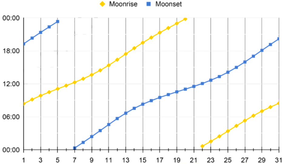
Solution: Do it yourself.
Class 8 Maths Ganita Prakash Solutions
- A Square and A Cube
- Power Play
- A Story of Numbers
- Quadrilaterals
- Number Play
- We Distribute Yet Things Multiply
- Proportional Reasoning-1
- Fractions In Disguise
- The Baudhayana-Pythagoras Theorem
- Proportional Reasoning-2
- Exploring Some Geometric Themes
- Tales by dots and lines
- Algebra Play

Test Generator
Create question paper PDF and online tests with your own name & logo in minutes.
Create Now
Learn8 App
Practice unlimited questions for Entrance tests & government job exams at ₹99 only
Install Now